-作者:JoeyQ
在上节 中,我们简单介绍了统计套利策略的原理,在本节中,我们将在沪深300各个行业中寻找可以配对的股票,并以此构造投资组合。投资组合更新的频率为每季度,我们主要步骤如下:
1.划分行业:在本研究中,我们主要研究的是银行,券商,医药,钢铁,煤炭,保险,房地产,家电,汽车制造这几个行业,概含了沪深300指数主要的行业
2.收益率相关性:我们选取的相关性阙值为0.7,太高导致价差波动小,太低则均值回归力度较弱。我们筛选出上一季度日收益率相关系数大于0.7的股票对作为备选股票
3.平稳性分析:在满足收益率相关系数大于0.7后,我们计算出价差,同时要求价差在0.05水平下通过单位根检验,这是为了防止上节中价差呈现单边走势的情况,我们要求价差必须围绕0轴波动
4.价差形态过滤:我们希望价差回归均值的速度较快,但由于我们调仓频率为一个季度,时间足够长,因此不需要通过这一步检验
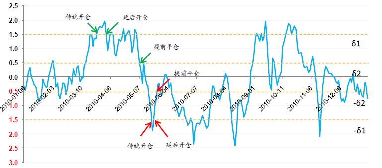
通过以上我们获得所有满足条件的股票对,并按照上一节的股票对交易策略进行交易,即当价差大于1.5时做多以单位A,同时做空$\beta$单位的B,当价差小于1.5时相反,当价差归零时清仓。我们测试了2007年至2017年的收益情况。结果如下:
可以发现我们获得一个很好的收益曲线!夏普值高达6.95!
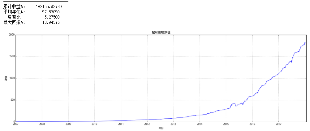
我们知道金融类股票的波动较小,因此我们剔除了银行,保险和券商股票,再构造投资组合,表现如下:
累计收益率显著提高,回撤控制在较小范围!
我们知道有左侧交易和右侧交易,左侧偏向反转,右侧偏向趋势,我们考虑建立配对交易策略的右侧交易策略,即当价差从上往下穿过1.5阙值线时建仓,同时,当价差趋向0时,回归均值的力度已经转弱,我们考虑价差小于0.5时清仓。具体流程如下:
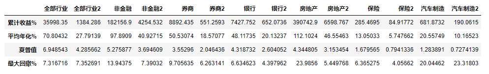
最后的最后,我们集中比较一下两种策略以及分行业的股票套利策略表现:
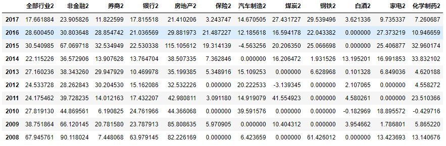
以下是近十年两种策略分行业的年度收益情况:
在这两节中,我们构造了统计套利之股票配对交易策略,并进行了沪深300行业的回测。我们假设所有的沪深300均可融资融券,从表现看我们的策略获得一个较为满意的收益,有效对冲了大盘下跌的风险。然而现实中并不是每只股票均可融资融券,因此这里可能存在未被市场参与者未能获取的超额收益。下一步,我们可以尝试针对可以融资融券的股票进行统计套利的回测!
import numpy as npimport pandas as pdimport matplotlib.pyplot as pltfrom scipy import statsimport statsmodels.api as smimport statsmodels.tsa.stattools as ts
##价差函数def get_jiacha(securityy, securityx,start_date,end_date):pricex=get_price(securityx,start_date,end_date,fields='close',fq='pre')['close']pricey=get_price(securityy,start_date,end_date,fields='close',fq='pre')['close']model = sm.OLS(log(pricey),log(pricex)).fit()slope=model.params[0]st1=log(pricey)-slope*log(pricex)st=(st1-mean(st1))/std(st1)return st,slope
def get_peidui(code_index,stocks,start_date,end_date,corrindex=0.7,stationindex=0.05): ### 获得配对股票 #####输入:行业或者概念的代码,总的股票池,开始时间,结束时间,相关系数阙值,平稳性阙值##输出:所有的配对股票,按照行业分类hangye=[] for i in arange(len(code_index)):tempt99=[i99 for i99 in get_concept_stocks(code_index[i]) if i99 in stocks]hangye.append(tempt99)store=[]allstore=[]##储存所有配对股票 for i56 in arange(len(hangye)):price=get_price(hangye[i56],start_date,end_date,fields='close')['close']##相关系数阙值for i in arange(len(price.columns)-1):for j in arange(i+1,len(price.columns)):if corrcoef(price[price.columns[i]],price[price.columns[j]])[0][1]>corrindex and \ts.adfuller(get_jiacha(price.columns[i],price.columns[j],start_date,end_date)[0],0)[1]<stationindex: ###平稳性检验以及相关性检验store.append([price.columns[i],price.columns[j]])allstore=allstore+storereturn allstore
def get_cumrate(allstore,start_date,end_date,jiacha_index=1.5):### 计算累计净值 #####输入:allstore所有的配对股票,开始时间,结束时间##输出:每个配对股票的净值bigstore=pd.DataFrame()if len(allstore)<1:bigstore['0']=[1 for i in arange(len(get_price('600001.XSHG',start_date,end_date))-2)]else:for j in arange(len(allstore)):##allstore长度price=get_price(allstore[j],start_date,end_date,fields='close',fq='pre')['close']st,slope=get_jiacha(allstore[j][0],allstore[j][1],start_date,end_date)u=0sec1=[] sec2=[]sec1num=0sec2num=0for i in arange(1,len(st)):if u==0 and st[i]>jiacha_index and st[i]<3:sec1num=-1##做空sec1sec2num=-sec1num*slope ##做多sec2u=ielif (u<>0 and st[i]*st[i-1]<0) or (abs(st[i])>3): ##此时价差变0清仓,或者价差偏离过大达到3清仓sec1num=0sec2num=0u=0elif u==0 and st[i]<-jiacha_index and st[i]>-3:sec1num=1sec2num=-sec1num*slopeu=isec1.append(sec1num)sec2.append(sec2num) #储存的是建仓信号,长度为price-1sec1rate=price[allstore[j][0]].diff(1)[1:]/list(price[allstore[j][0]][:-1])sec2rate=price[allstore[j][1]].diff(1)[1:]/list(price[allstore[j][1]][:-1])sumrate=sec1rate[1:]*sec1[:-1]+sec2rate[1:]*sec2[:-1] #发出信号后一天建仓cumrate=[]tempt=1for i in arange(len(sumrate)):tempt=tempt*(1+sumrate[i])if sumrate[i-1]<>0:tempt=tempt*(1-0.01/255)##融券费用if i >=1:if sumrate[i-1]<>0 and sumrate[i]==0:tempt=tempt*(1-0.001-0.00025) ##平仓手续费 cumrate.append(tempt)#plt.plot(cumrate)#plt.title('配对策略净值变化曲线')bigstore[j]=cumratereturn bigstoredef trade(code_index,stocks,time,plot_index=True,print_index=True):###交易函数 #####输入:行业代码,股票池,时间##输出:净值曲线,总收益,年化收益,夏普比,最大回撤netvalue=[]##储存净值tempt22=1nianhua=[]##储存年末净值for ii11 in arange(len(time)-2):allstore=get_peidui(code_index,stocks,start_date=time[ii11],end_date=time[ii11+1])##获得配对bigstore=get_cumrate(allstore,start_date=time[ii11+1],end_date=time[ii11+2])tempt23=[ii77*tempt22 for ii77 in list(bigstore.mean(axis=1))]netvalue=netvalue+tempt23tempt22=netvalue[-1]nianhua.append(netvalue[-1])###绘制净值图像if plot_index==True:plt.figure(figsize=(20,6))plt.plot(netvalue)timestamp=[time[i*4][:4] for i in arange(len(time)/4)]plt.xticks(np.arange(0,len(netvalue),len(netvalue)/len(timestamp)),timestamp)plt.grid(True)plt.title('配对策略净值')plt.xlabel('年份')plt.ylabel('净值')###计算最大回撤,平均年化收益率,夏普比tt1=[]tt2=[]for i in arange(len(netvalue)):for j in arange(i+1,len(netvalue)):tt1.append((netvalue[i]-netvalue[j])/netvalue[i])tt2.append(max(tt1))huiche=max(tt2)*100 #最大回撤yearrate=[nianhua[i]/nianhua[i-1]-1 for i in arange(1,len(nianhua))]shouyi=[netvalue[ii88+1]/netvalue[ii88]-1 for ii88 in arange(len(netvalue)-1) ]#每日收益sharpe=(mean(shouyi)-0.0285/252)/std(shouyi)*np.sqrt(252)#夏普值#sharpe=(mean(yearrate)-0.04)/std(yearrate) pjnh=((netvalue[-1])**(1./(len(time)/4))-1)*100 #平均年化ljnh=(netvalue[-1]-1)*100 #累计收益##打印if print_index==True:print '-'*30print '%14s %15.5f' % ('累计收益%:',ljnh)print '%14s %15.5f' % ('平均年化%:',pjnh)print '%14s %15.5f' % ('夏普比:' , sharpe)print '%14s %15.5f' % ('最大回撤%:', huiche)##返回一些数值进行对比:累计收益,平均年化,夏普值,最大回撤,年末净值return [ljnh,pjnh,sharpe,huiche,nianhua]##获取沪深300分行业股票数据##券商:GN780,银行:GN815,房地产GN733,保险GN646,汽车制造GN835,煤炭GN823,钢铁GN727,白酒GN705,家电GN706,化学制药GN750stocks = get_index_stocks('000300.XSHG')hangye=[]code_index=['GN780','GN815','GN733','GN646','GN835','GN823','GN727','GN705','GN706','GN750']for i in arange(len(code_index)):tempt99=[i99 for i99 in get_concept_stocks(code_index[i]) if i99 in stocks]hangye.append(tempt99)###按照季度生成时间time=[]for i in arange(2007,2018):for j in arange(1,13,3):time.append(str(i)+'-'+str(j)+'-01')
##储存输出指标storeindex=pd.DataFrame()##进行交易storeindex['全部行业']=trade(code_index,stocks,time)
累计收益%:     35998.35195
平均年化%:        70.80432
  夏普比:         6.94854
最大回撤%:         7.31672
##根据经验我们知道银行,保险,券商等金融类股票波动较小,我们把他们剔除后看他们的配对交易收益storeindex['非金融']=trade(['GN733','GN835','GN823','GN727','GN705','GN706','GN750'],stocks,time)
累计收益%:    182156.93730
平均年化%:        97.89090
  夏普比:         5.27588
最大回撤%:        13.94375
##分行业计算相关指标storeindex['券商']=trade(['GN780'],stocks,time,print_index=False,plot_index=False)storeindex['银行']=trade(['GN815'],stocks,time,print_index=False,plot_index=False)storeindex['房地产']=trade(['GN733'],stocks,time,print_index=False,plot_index=False)storeindex['保险']=trade(['GN646'],stocks,time,print_index=False,plot_index=False)storeindex['汽车制造']=trade(['GN835'],stocks,time,print_index=False,plot_index=False)storeindex['煤炭']=trade(['GN823'],stocks,time,print_index=False,plot_index=False)storeindex['钢铁']=trade(['GN727'],stocks,time,print_index=False,plot_index=False)storeindex['白酒']=trade(['GN705'],stocks,time,print_index=False,plot_index=False)storeindex['家电']=trade(['GN706'],stocks,time,print_index=False,plot_index=False)storeindex['化学制药']=trade(['GN750'],stocks,time,print_index=False,plot_index=False)
def get_cumrate2(allstore,start_date,end_date,jiacha_index=1.5):### 计算累计净值 #####输入:allstore所有的配对股票,开始时间,结束时间##输出:每个配对股票的净值bigstore=pd.DataFrame()if len(allstore)<1:bigstore['0']=[1 for i in arange(len(get_price('600001.XSHG',start_date,end_date))-2)]else:for j in arange(len(allstore)):##allstore长度price=get_price(allstore[j],start_date,end_date,fields='close',fq='pre')['close']st,slope=get_jiacha(allstore[j][0],allstore[j][1],start_date,end_date)u=0sec1=[] sec2=[]sec1num=0sec2num=0for i in arange(1,len(st)):if u==0 and st[i-1]>jiacha_index and st[i]<jiacha_index: ##从上往下穿过1.5时开仓sec1num=-1##做空sec1sec2num=-sec1num*slope ##做多sec2u=ielif (u<>0 and abs(st[i-1])>0.5 and abs(st[i])<0.5) or (abs(st[i])>3): ##此时价差变0清仓,或者价差偏离过大达到3清仓sec1num=0sec2num=0u=0elif u==0 and st[i-1]<-jiacha_index and st[i]>-jiacha_index: ##从下往上穿过1.5时开仓sec1num=1sec2num=-sec1num*slopeu=isec1.append(sec1num)sec2.append(sec2num) #储存的是建仓信号,长度为price-1sec1rate=price[allstore[j][0]].diff(1)[1:]/list(price[allstore[j][0]][:-1])sec2rate=price[allstore[j][1]].diff(1)[1:]/list(price[allstore[j][1]][:-1])sumrate=sec1rate[1:]*sec1[:-1]+sec2rate[1:]*sec2[:-1] #发出信号后一天建仓cumrate=[]tempt=1for i in arange(len(sumrate)):tempt=tempt*(1+sumrate[i])if i >=1:if sumrate[i-1]<>0:tempt=tempt*(1-0.01/250)##融券费用if sumrate[i]==0:tempt=tempt*(1-0.001-0.00025) ##交易费用cumrate.append(tempt)#plt.plot(cumrate)#plt.title('配对策略净值变化曲线')bigstore[j]=cumratereturn bigstoredef trade2(code_index,stocks,time,plot_index=True,print_index=True):###交易函数2 #####输入:行业代码,股票池,时间##输出:净值曲线,总收益,年化收益,夏普比,最大回撤netvalue=[]##储存净值tempt22=1nianhua=[]##储存年末净值for ii11 in arange(len(time)-2):allstore=get_peidui(code_index,stocks,start_date=time[ii11],end_date=time[ii11+1])##获得配对bigstore=get_cumrate2(allstore,start_date=time[ii11+1],end_date=time[ii11+2])tempt23=[ii77*tempt22 for ii77 in list(bigstore.mean(axis=1))]netvalue=netvalue+tempt23tempt22=netvalue[-1]nianhua.append(netvalue[-1])###绘制净值图像if plot_index==True:plt.figure(figsize=(20,6))plt.plot(netvalue)timestamp=[time[i*4][:4] for i in arange(len(time)/4)]plt.xticks(np.arange(0,len(netvalue),len(netvalue)/len(timestamp)),timestamp)plt.grid(True)plt.title('配对策略净值')plt.xlabel('年份')plt.ylabel('净值')###计算最大回撤,平均年化收益率,夏普比tt1=[]tt2=[]for i in arange(len(netvalue)):for j in arange(i+1,len(netvalue)):tt1.append((netvalue[i]-netvalue[j])/netvalue[i])tt2.append(max(tt1))huiche=max(tt2)*100 #最大回撤yearrate=[nianhua[i]/nianhua[i-1]-1 for i in arange(1,len(nianhua))]shouyi=[netvalue[ii88+1]/netvalue[ii88]-1 for ii88 in arange(len(netvalue)-1) ]#每日收益sharpe=(mean(shouyi)-0.0285/252)/std(shouyi)*np.sqrt(250)#夏普值pjnh=((netvalue[-1])**(1./(len(time)/4))-1)*100 #平均年化ljnh=(netvalue[-1]-1)*100 #累计收益##打印if print_index==True:print '-'*30print '%14s %15.5f' % ('累计收益%:',ljnh)print '%14s %15.5f' % ('平均年化%:',pjnh)print '%14s %15.5f' % ('夏普比:' , sharpe)print '%14s %15.5f' % ('最大回撤%:', huiche)##返回一些数值进行对比:累计收益,平均年化,夏普值,最大回撤,年净值return [ljnh,pjnh,sharpe,huiche,nianhua]##进行新的策略交易storeindex['全部行业2']=trade2(code_index,stocks,time,print_index=False,plot_index=False)storeindex['非金融2']=trade2(['GN733','GN835','GN823','GN727','GN705','GN706','GN750'],stocks,time,print_index=False,plot_index=False)storeindex['券商2']=trade2(['GN780'],stocks,time,print_index=False,plot_index=False)storeindex['银行2']=trade2(['GN815'],stocks,time,print_index=False,plot_index=False)storeindex['房地产2']=trade2(['GN733'],stocks,time,print_index=False,plot_index=False)storeindex['保险2']=trade2(['GN646'],stocks,time,print_index=False,plot_index=False)storeindex['汽车制造2']=trade2(['GN835'],stocks,time,print_index=False,plot_index=False)storeindex['煤炭2']=trade2(['GN823'],stocks,time,print_index=False,plot_index=False)storeindex['钢铁2']=trade2(['GN727'],stocks,time,print_index=False,plot_index=False)storeindex['白酒2']=trade2(['GN705'],stocks,time,print_index=False,plot_index=False)storeindex['家电2']=trade2(['GN706'],stocks,time,print_index=False,plot_index=False)storeindex['化学制药2']=trade2(['GN750'],stocks,time,print_index=False,plot_index=False)
storeindex1=storeindex
##更改行名,同时计算每年的收益storeindex1.index=['累计收益%','平均年化%','夏普值','最大回撤%','年净值']##计算每年收益shinianrate=pd.DataFrame()for ii67 in arange(len(storeindex1.columns)): uiu=[(storeindex1.iloc[-1][ii67][-1-4*i]/storeindex1.iloc[-1][ii67][-1-4*(i+1)]-1)*100 for i in arange(10)] #2008-2018年化收益shinianrate[storeindex1.columns[ii67]]=uiushinianrate.index=[str(ii864) for ii864 in arange(2017,2007,-1)]
###比较一下改进的策略和未改进策略##生成交错的index【0,12,1,13...】tempt776=[]for i776 in arange(12):tempt776=tempt776+[i776,i776+12]
| 全部行业 | 全部行业2 | 非金融 | 非金融2 | 券商 | 券商2 | 银行 | 银行2 | 房地产 | 房地产2 | 保险 | 保险2 | 汽车制造 | 汽车制造2 | |
|---|---|---|---|---|---|---|---|---|---|---|---|---|---|---|
| 累计收益% | 35998.35 | 1384.286 | 182156.9 | 4254.532 | 8892.435 | 551.2593 | 7427.752 | 652.0736 | 390742.9 | 6598.767 | 285.4695 | 84.91772 | 681.8732 | 190.0615 |
| 平均年化% | 70.80432 | 27.79139 | 97.8909 | 40.92715 | 50.53074 | 18.57077 | 48.11735 | 20.13237 | 112.1024 | 46.55463 | 13.05033 | 5.747662 | 20.55749 | 10.16523 |
| 夏普值 | 6.948543 | 4.285662 | 5.275877 | 3.694609 | 3.55296 | 2.046436 | 4.318732 | 2.604052 | 4.344805 | 3.153454 | 1.679565 | 0.7941336 | 1.283891 | 0.7274139 |
| 最大回撤% | 7.316716 | 7.352691 | 13.94375 | 7.39032 | 9.705635 | 6.263141 | 6.634623 | 4.397962 | 23.9856 | 5.449768 | 6.365275 | 4.05662 | 20.04462 | 23.31803 |
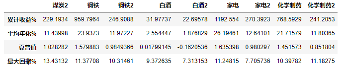
storeindex1[:-1].iloc[:,tempt776[15:24]]
| 煤炭2 | 钢铁 | 钢铁2 | 白酒 | 白酒2 | 家电 | 家电2 | 化学制药 | 化学制药2 | |
|---|---|---|---|---|---|---|---|---|---|
| 累计收益% | 229.1934 | 959.7964 | 246.9088 | 31.97737 | 22.69578 | 1192.554 | 270.3923 | 768.5929 | 241.2053 |
| 平均年化% | 11.43998 | 23.9373 | 11.97227 | 2.554447 | 1.876829 | 26.19461 | 12.64101 | 21.71579 | 11.80365 |
| 夏普值 | 1.028282 | 1.579883 | 0.9849366 | 0.01799145 | -0.1620536 | 1.635398 | 0.980297 | 1.451573 | 0.851804 |
| 最大回撤% | 13.43132 | 11.37708 | 10.31461 | 9.372635 | 7.313153 | 11.24815 | 7.705736 | 10.39782 | 11.18275 |
###近十年各行业标准策略每年收益率情况shinianrate.iloc[:,:11]
| 全部行业 | 非金融 | 券商 | 银行 | 房地产 | 保险 | 汽车制造 | 煤炭 | 钢铁 | 白酒 | 家电 | |
|---|---|---|---|---|---|---|---|---|---|---|---|
| 2017 | 43.374497 | 67.715375 | 31.157004 | 37.220780 | 68.051485 | 11.908842 | 23.832291 | 60.676597 | 42.554389 | 8.681982 | 16.828608 |
| 2016 | 73.045802 | 87.606505 | 73.237407 | 47.931498 | 92.702984 | 44.694205 | 24.390914 | 36.163588 | 56.680092 | 0.000000 | 42.157159 |
| 2015 | 87.413288 | 114.068589 | 118.418676 | 70.680948 | 182.131038 | 46.848888 | 8.490181 | 18.967875 | 68.813437 | 0.000000 | 99.501733 |
| 2014 | 54.252412 | 91.913083 | 28.972415 | 40.647905 | 100.088921 | 17.571398 | 0.000000 | 30.719199 | 2.870304 | 21.370870 | 27.710186 |
| 2013 | 68.430184 | 99.139680 | 81.430820 | 27.559198 | 98.463189 | 20.675230 | 19.176097 | 0.000000 | 22.277904 | 1.972493 | 12.245891 |
| 2012 | 62.124883 | 62.161048 | 85.660451 | 37.756974 | 72.977620 | 0.000000 | 31.602411 | 1.104353 | 0.000000 | 1.196550 | 0.000000 |
| 2011 | 68.659565 | 103.500942 | 49.248848 | 43.269864 | 115.175938 | 7.640108 | 47.879670 | 94.068395 | 0.000000 | -1.331203 | -1.518100 |
| 2010 | 71.673487 | 113.963463 | 19.938291 | 55.386869 | 112.454515 | 0.000000 | 93.859601 | 0.000000 | 0.000000 | 3.554363 | 47.479586 |
| 2009 | 115.378049 | 222.437618 | 57.715104 | 53.991063 | 295.856777 | 6.147531 | 0.000000 | 35.539289 | 0.000000 | -0.939281 | 12.132745 |
| 2008 | 144.392647 | 167.743005 | 12.816298 | 156.434453 | 158.712859 | 0.000000 | 4.057777 | 0.000000 | 123.451360 | 0.000000 | 17.749064 |
###近十年各行业每年收益率情况shinianrate.iloc[:,12:]
| 全部行业2 | 非金融2 | 券商2 | 银行2 | 房地产2 | 保险2 | 汽车制造2 | 煤炭2 | 钢铁2 | 白酒2 | 家电2 | 化学制药2 | |
|---|---|---|---|---|---|---|---|---|---|---|---|---|
| 2017 | 17.661884 | 23.905826 | 11.822599 | 17.815518 | 21.410206 | 3.243747 | 14.670505 | 27.431727 | 29.539496 | 3.621336 | 9.735337 | 7.260687 |
| 2016 | 28.600450 | 30.803648 | 28.854742 | 21.036569 | 29.881973 | 21.487227 | 12.185618 | 16.594178 | 22.043382 | 0.000000 | 27.373219 | 10.946659 |
| 2015 | 30.540985 | 67.069718 | 32.534949 | 22.530338 | 115.105612 | 19.314139 | -4.563256 | 20.206350 | 25.066698 | 0.000000 | 25.406877 | 32.960174 |
| 2014 | 22.115226 | 36.572906 | 13.907628 | 13.764704 | 38.507335 | 7.362846 | 0.000000 | 16.206472 | 1.931526 | 13.195201 | 16.991853 | 33.832102 |
| 2013 | 27.160236 | 38.343260 | 29.947929 | 10.469978 | 35.199385 | 5.348916 | 15.109253 | 0.000000 | 6.628968 | 0.101328 | 6.849036 | 4.620188 |
| 2012 | 24.533728 | 28.262843 | 30.204530 | 15.162086 | 32.532226 | 0.000000 | 20.222533 | -3.139345 | 0.000000 | 2.107065 | 0.000000 | 4.558272 |
| 2011 | 24.175462 | 39.728235 | 14.012163 | 17.432207 | 42.980811 | 3.091180 | 14.919079 | 41.554923 | 0.000000 | 4.580261 | 0.000000 | 23.510366 |
| 2010 | 27.819130 | 44.869561 | 6.190825 | 24.761966 | 44.366068 | 0.000000 | 39.591576 | 0.000000 | 0.000000 | -0.182969 | 18.895572 | -0.429716 |
| 2009 | 38.751864 | 66.120145 | 20.781580 | 23.787913 | 85.808635 | 5.970905 | 0.000000 | 10.404312 | 0.000000 | 3.954662 | 1.786801 | 5.865220 |
| 2008 | 67.945761 | 90.118024 | 7.448068 | 63.979145 | 82.226169 | 0.000000 | 6.423659 | 0.000000 | 61.426012 | 0.000000 | 13.423693 | 13.140676 |

本社区仅针对特定人员开放
查看需注册登录并通过风险意识测评
5秒后跳转登录页面...
移动端课程