1、研究内容：

本文主要研究内容是基于rank IC分析医疗板块四大类因子（风格类、技术类、盈利能力类、基本面类）盈利预测能力，以及在此基础上构建医疗板块多因子rank IC赋权模型。
本文将分为以下三个板块：
1、因子选取及数据预处理
2、医疗板块因子分析
3、构建医疗板块多因子模型
本文内容较为基础，另附单行业因子研究及单行业rank IC多因子模型回测代码。

2、因子选取及数据预处理：

2.1、因子选取

本文基于海通证券研报的内容，选取四大类因子（风格类、技术类、盈利能力类、基本面类）作为所选研究因子。具体如下表：

2.2、数据预处理

股票池：申万一级医疗行业中非*ST股
时间维度：2010年1月1日——2018年8月1日
处理方式：去空值、去极值、中性化、标准化
（1）、去空值：先将任一因子数据全部为空的股票从股票池中剔除，再将剩余股票的空值用当天医药行业该因子的平均水平进行填充。
（2）、去极值：采取中位数去极值法
（3）、中性化：将除了市值外的因子对市值进行中性化。因为股票池全部为同一行业的股票。无需对行业哑变量进行中性化。
（4）、标准化：采取传统均值标准化方法

3、医疗板块因子分析

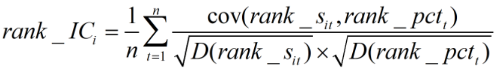
本文的因子分析方式为rank IC均值分析法。rank IC是分析因子有效性的常用指标。

3.1、rank IC介绍

因子IC的求解方式为：时间维度上因子与股票收益率相关系数的均值。因子rank IC求解原理与IC相同，不同的仅在于其使用的数据是因子在股票池中的排名而非其数值。这样的做法能够在统计学中避免很多问题，数值效果也更为有效。
具体公式如下：
t：日期
n：日期总数
rank_Sit：第i个因子在第t天的数据向量
rank_PCTt：第t天的股票收益率数据向量
rank_ICi：第i个因子的IC均值

3.2、医疗行业因子IC分析

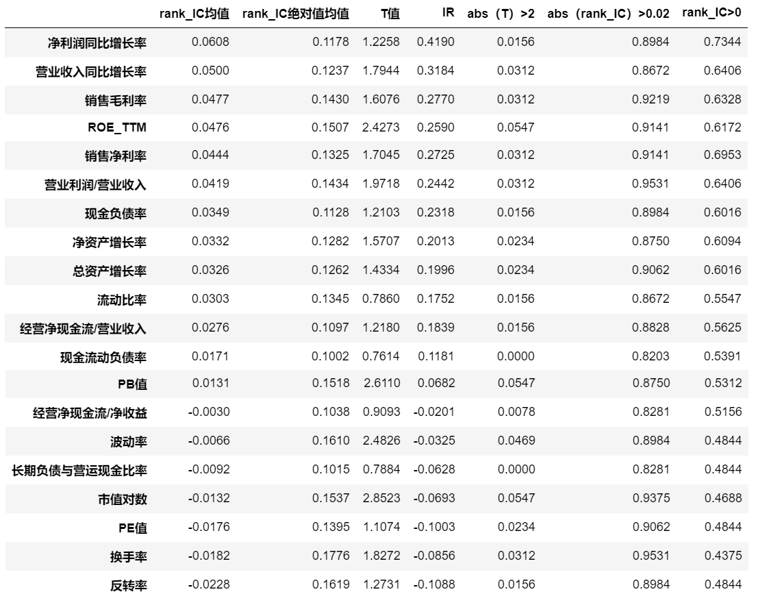
医疗板块因子分析的结果汇总如下表：

可以很明显的看到：对于医药板块而言，部分基本面因子仍然有十分出色的表现。盈利能力因子（ROE）表现也十分出色。换手率、反转率等技术面因子与股票收益率有显著的反向相关关系。
而其中需要注意的是风格类因子：市值、PE和PB的rank IC表现并不出色。但如果将其与股票收益率做回归的话会发现R方仍然很高。其原因是17年后市值因子等出现反转，在17年前市值与股票收益反向相关而17年后变成正向相关，从而使得rank IC均值降低。因此我又测算了rank IC绝对值的均值，发现风格类因子的绝对值均值仍保持在较高水平，说明风格类因子仍然时有效的。

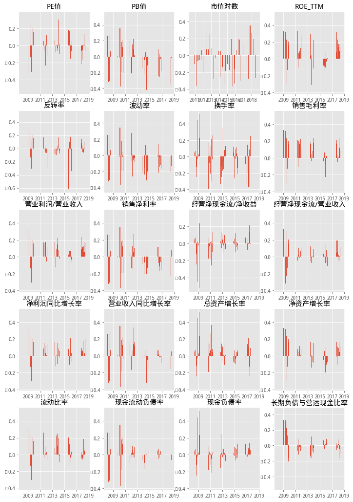
不同因子随时间的IC值如下：

可以看出：风格类因子（典型如PB值、市值对数）在后期逐渐出现反转趋势。技术类因子与收益率大体呈反向关系。基本面因子中，销售毛利率、净利润同比增长率、销售净利率等具有出色表现，而经营净现金流/净收益、经营净现金流/营业收入等效果不显著。

4、构建医疗板块多因子模型：

根据研报内容，本文先通过逐步筛选法筛选出选股效果最为显著的因子，然后通过因子在不同时间段的rank IC值对因子进行赋权，形成新的组合因子。通过组合因子进行选股。

4.1、逐步筛选法：

筛选因子过程中，本文采用了线性回归WLS模型。
模型将股票收益率看做是能用若干因子作为自变量的WLS线性回归模型进行解释的因变量。
本文通过以下筛选条件筛选因子：
条件一：已选因子f的WLS模型系数显著
条件二：在满足条件一的备选因子中，因子f能使模型新增调整R方最大
本文通过以上条件，筛选出如下的因子表：
显著性水平=0.2：
PB值、市值对数、换手率、ROE
显著性水平=0.3：
PB值、市值对数、换手率、ROE、销售毛利率、营业收入同比增长率、营业利润/营业收入

4.2、多因子模型：

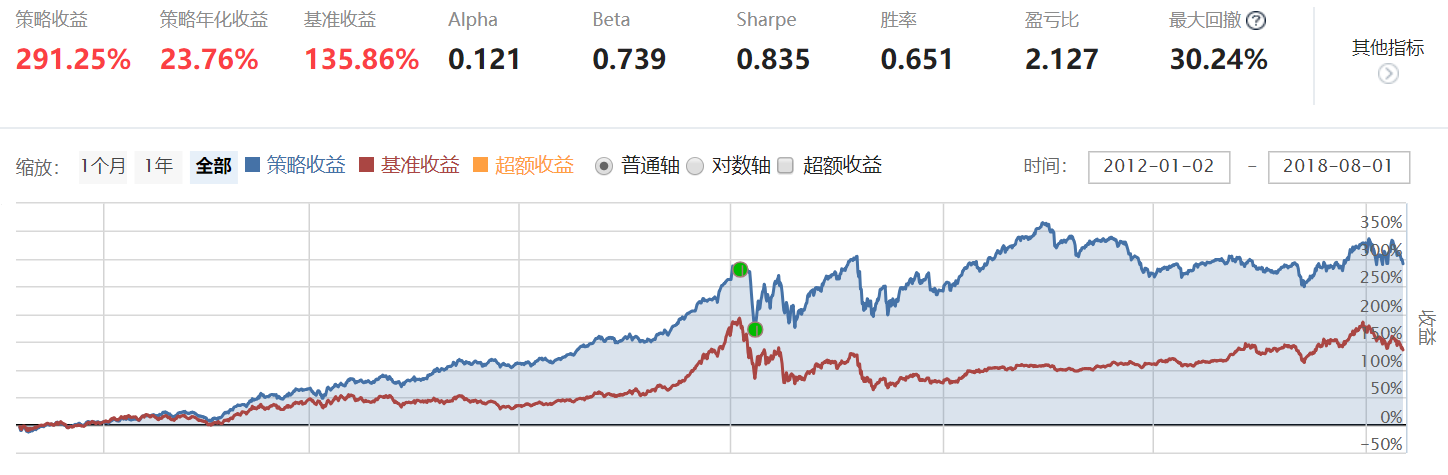
通过以上所选因子，*新的组合因子。因子的权重为学习周期内各因子的IC均值。然后选取组合因子分数最高的20只股票构建等权组合。
具体参数：
调仓周期：1个月
学习周期：12个月
购买股票数量：20
回测周期：2010年1月1日——2018年8月1日
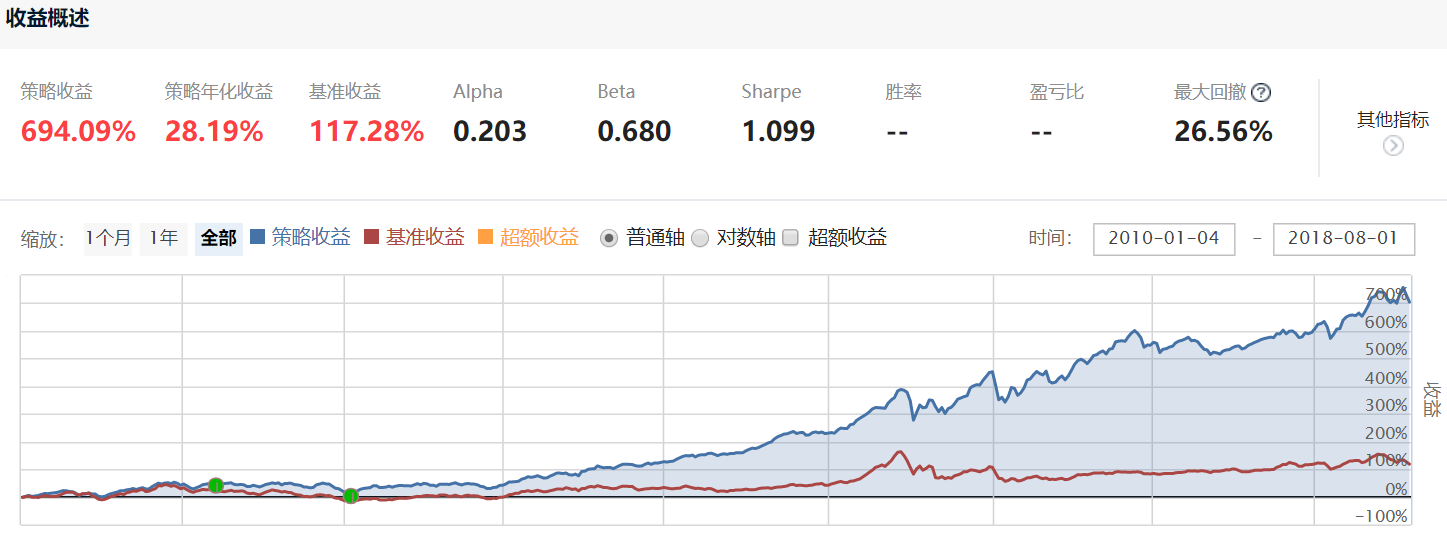
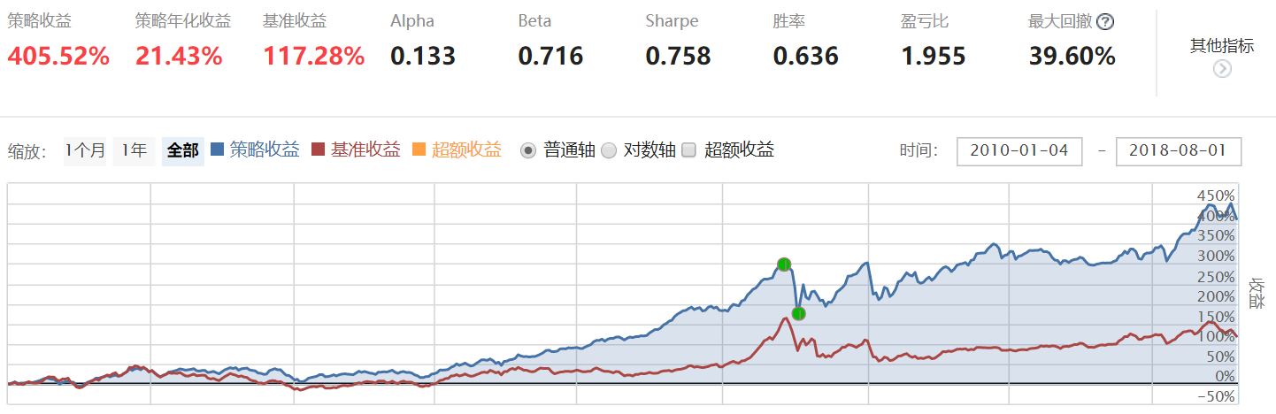
因子池：显著性水平=0.2的因子（显著性水平=0.3的因子也有测试，收益率相差不大但是最大回撤会放大）
在测试中，学习周期为24个月的回测结果不如学习周期为12个月的回测结果。


学习周期为6个月的回测结果也不如学习周期为12个月的回测结果。

该模型策略年化收益达到28.19%，也具有较为明显的超额收益。

5、总结：

常见选股因子在医药行业内存在显著选股效果。风格类因子收益高但稳定性较差，从17年后存在反转趋势。技术类因子较为有效，与收益率呈显著负相关性。基本面因子则部分有效部分不有效。总体而言，企业盈利能力越高，资产增长越快，利润增长越快，盈利质量越好，偿债能力越强，股票收益表现越优。

import timefrom datetime import datetime, timedeltaimport jqdatafrom jqdata import *from jqdata import financeimport numpy as npimport pandas as pdimport mathfrom sklearn.decomposition import PCAfrom itertools import combinationsfrom statsmodels import regressionimport statsmodels.api as smimport matplotlib.pyplot as pltfrom jqfactor import get_factor_valuesimport datetimefrom jqlib.technical_analysis import *from scipy import statsfrom sklearn.linear_model import Ridgefrom sklearn.preprocessing import Imputerfrom jqfactor import winsorize_medfrom jqfactor import neutralizefrom jqfactor import standardlize#设置画图样式plt.style.use('ggplot')#输入起止日期，返回所有自然日日期def get_date_list(begin_date, end_date):dates = []dt = datetime.strptime(begin_date,"%Y-%m-%d")date = begin_date[:]while date <= end_date:dates.append(date)dt += timedelta(days=1)date = dt.strftime("%Y-%m-%d")return dates#去极值函数#mad中位数去极值法def filter_extreme_MAD(series,n): #MAD: 中位数去极值 median = series.quantile(0.5)new_median = ((series - median).abs()).quantile(0.50)max_range = median + n*new_medianmin_range = median - n*new_medianreturn np.clip(series,min_range,max_range)#进行标准化处理def winsorize(factor, std=3, h*e_negative = True):'''    去极值函数     factor:以股票code为index，因子值为value的Series    std为几倍的标准差，h*e_negative 为布尔值，是否包括负值    输出Series    '''r=factor.dropna().copy()if h*e_negative == False:r = r[r>=0]else:pass#取极值edge_up = r.mean()+std*r.std()edge_low = r.mean()-std*r.std()r[r>edge_up] = edge_upr[r<edge_low] = edge_lowreturn r#标准化函数：def standardize(s,ty=2):'''    s为Series数据    ty为标准化类型:1 MinMax,2 Standard,3 maxabs     '''data=s.dropna().copy()if int(ty)==1:re = (data - data.min())/(data.max() - data.min())elif ty==2:std = data.std()if std==0:std = 1re = (data - data.mean())/stdelif ty==3:re = data/10**np.ceil(np.log10(data.abs().max()))return re#正交化函数def new_zj(A):T=len(A[:,0])K=len(A[0,:])fmean=np.zeros_like(A)FF=np.zeros_like(A)tzg=np.zeros((K,K))for i in arange(K):fmean[:,i]=A[:,i]-mean(A[:,i])fmean=mat(fmean)M=(T-1)*numpy.cov(fmean.T) #获得重叠矩阵M=mat(M)u,v=np.linalg.eig(M) #u是特征值，v是特征向量sk1=np.dot( np.dot(v ,np.linalg.inv(np.diag(u**0.5)) ), v.T)sk2=np.dot(sk1*((T-1)**0.5),np.diag(A.var(axis=0)**0.5))####F=np.dot(A,sk2)for i in arange(K):FF[:,i]=[float(j) for j in F[:,i]]return FFdef get_zj(target_factor,minor_factor,pl_pro):zj_factor_list = [minor_factor,target_factor]zj_list = []for j in range(0,len(zj_factor_list)):zj_list.append(zj_factor_list[j]+'_zj')df = pd.DataFrame(columns = pl_pro.minor_axis)for i in range(0,len(pl_pro.major_axis)):A_df = pd.DataFrame(index = pl_pro.minor_axis)for j in range(0,len(zj_factor_list)):A_df[zj_factor_list[j]] = pl_pro[zj_factor_list[j]].iloc[i,:]A = A_df.as_matrix()A_f = new_zj(A)df[pl_pro.major_axis[i]] = A_f[:,1]pl_pro[zj_list[1]] = df#中性化函数#传入：mkt_cap：以股票为index，市值为value的Series,#factor：以股票code为index，因子值为value的Series,#输出：中性化后的因子值seriesdef neutralization(factor,mkt_cap = False, industry = False):y = factorif type(mkt_cap) == pd.Series:#LnMktCap = mkt_cap.apply(lambda x:math.log(x))if industry: #行业、市值dummy_industry = get_industry_exposure(factor.index)x = pd.concat([mkt_cap,dummy_industry.T],axis = 1)else: #仅市值x = mkt_capelif industry: #仅行业dummy_industry = get_industry_exposure(factor.index)x = dummy_industry.Tresult = sm.OLS(y.astype(float),x.astype(float)).fit()return result.resid#为股票池添加行业标记,return df格式 ,为中性化函数的子函数   def get_industry_exposure(stock_list):df = pd.DataFrame(index=jqdata.get_industries(name='sw_l1').index, columns=stock_list)for stock in stock_list:try:df[stock][get_industry_code_from_security(stock)] = 1except:continuereturn df.fillna(0)#将NaN赋为0#查询个股所在行业函数代码（申万一级） ,为中性化函数的子函数    def get_industry_code_from_security(security,date=None):industry_index=jqdata.get_industries(name='sw_l1').indexfor i in range(0,len(industry_index)):try:index = get_industry_stocks(industry_index[i],date=date).index(security)return industry_index[i]except:continuereturn u'未找到'    def get_win_stand_neutra(stocks):h=get_fundamentals(query(valuation.pb_ratio,valuation.code,valuation.market_cap)\.filter(valuation.code.in_(stocks)))stocks_pb_se=pd.Series(list(h.pb_ratio),index=list(h.code))stocks_pb_win_standse=standardize(winsorize(stocks_pb_se))stocks_mktcap_se=pd.Series(list(h.market_cap),index=list(h.code))stocks_neutra_se=neutralization(stocks_pb_win_standse,stocks_mktcap_se)return stocks_neutra_se #获取日期列表def get_tradeday_list(start,end,frequency=None,count=None):if count != None:df = get_price('000001.XSHG',end_date=end,count=count)else:df = get_price('000001.XSHG',start_date=start,end_date=end)if frequency == None or frequency =='day':return df.indexelse:df['year-month'] = [str(i)[0:7] for i in df.index]if frequency == 'month':return df.drop_duplicates('year-month').indexelif frequency == 'quarter':df['month'] = [str(i)[5:7] for i in df.index]df = df[(df['month']=='01') | (df['month']=='04') | (df['month']=='07') | (df['month']=='10') ]return df.drop_duplicates('year-month').indexelif frequency =='halfyear':df['month'] = [str(i)[5:7] for i in df.index]df = df[(df['month']=='01') | (df['month']=='06')]return df.drop_duplicates('year-month').index 
        def ret_se(start_date='2018-6-1',end_date='2018-7-1',stock_pool=None,weight=0):pool = stock_poolif len(pool) != 0:#得到股票的历史价格数据df = get_price(list(pool),start_date=start_date,end_date=end_date,fields=['close']).closedate_list = list(df.index)for i in range(len(df.index)):mean = np.nanmean(np.array(df.iloc[i,:]))df.iloc[i,:] = df.iloc[i,:].fillna(mean)#df = df.dropna(axis=1)#获取列表中的股票流通市值对数值df_mkt = get_fundamentals(query(valuation.code,valuation.circulating_market_cap).filter(valuation.code.in_(df.columns)))df_mkt.index = df_mkt['code'].valuesfact_se =pd.Series(df_mkt['circulating_market_cap'].values,index = df_mkt['code'].values)fact_se = np.log(fact_se)else:df = get_price('000001.XSHG',start_date=start_date,end_date=end_date,fields=['close'])df['v'] = [1]*len(df)del df['close']#相当于昨天的百分比变化pct = df.pct_change()+1pct.iloc[0,:] = 1if weight == 0:#等权重平均收益结果#print (pct.cumsum(axis=1))se = pct.cumsum(axis=1).iloc[:,-1]/pct.shape[1]return seelse:#按权重的方式计算se = (pct*fact_se).cumsum(axis=1).iloc[:,-1]/sum(fact_se)return se#获取所有分组pct，默认为5组def get_all_pct(pool_dict,trade_list,groups=5):num = 1for s,e in zip(trade_list[:-1],trade_list[1:]):stock_list = pool_dict[s]stock_num = len(stock_list)//groupsif num == 0:pct_se_list = []for i in range(groups):temp = ret_se(start_date=s,end_date=e,stock_pool=stock_list[i*stock_num:(i+1)*stock_num])pct_se_list.append(temp)pct_df1 = pd.concat(pct_se_list,axis=1)pct_df = pd.concat([pct_df,pct_df1],axis=0)else:pct_se_list = []for i in range(groups):pct_se_list.append(ret_se(start_date=s,end_date=e,stock_pool=stock_list[i*stock_num:(i+1)*stock_num]))pct_df = pd.concat(pct_se_list,axis=1)    num = 0return pct_df#获取指定交易日往前推count天交易日def tradedays_before(date,count):date = get_price('000001.XSHG',end_date=date,count=count+1).index[0]return date#去空值，用行业平均值代替def get_key (dict, value):return [k for k, v in dict.items() if v == value]def replace_nan_indu(factor_data,stockList,industry_code,date):#把nan用行业平均值代替，依然会有nan，此时用所有股票平均值代替i_Constituent_Stocks={}if isinstance(factor_data,pd.DataFrame):data_temp=pd.DataFrame(index=industry_code,columns=factor_data.columns)for i in industry_code:temp = get_industry_stocks(i, date)i_Constituent_Stocks[i] = list(set(temp).intersection(set(stockList)))data_temp.loc[i]=mean(factor_data.loc[i_Constituent_Stocks[i],:])for factor in data_temp.columns:#行业缺失值用所有行业平均值代替null_industry=list(data_temp.loc[pd.isnull(data_temp[factor]),factor].keys())for i in null_industry:data_temp.loc[i,factor]=mean(data_temp[factor])null_stock=list(factor_data.loc[pd.isnull(factor_data[factor]),factor].keys())for i in null_stock:industry=get_key(i_Constituent_Stocks,i)if industry:factor_data.loc[i,factor]=data_temp.loc[industry[0],factor] else:factor_data.loc[i,factor]=mean(factor_data[factor])return factor_data#去空值，用行业平均值代替def delete_nan(factor_list,pl_pro,key=1):if key==1:pl_new = pl_pro.copy()#将某个因子全为空的股票剔除pl_new.replace(np.inf,np.nan,inplace=True)for i in range(1,len(factor_list)):t=0while t<len(pl_new[factor_list[i]].columns):if pl_new[factor_list[i]].iloc[:,t].isnull().all()==True:pl_new.drop([pl_new[factor_list[i]].columns[t]],axis=2,inplace=True)else:label = 0ss = pl_new[factor_list[i]].iloc[0,t]for b in range(1,len(pl_new[factor_list[i]].index)):if pl_new[factor_list[i]].iloc[b,t] == ss:continueelse:label = 1breakif label==0:pl_new.drop([pl_new[factor_list[i]].columns[t]],axis=2,inplace=True)else:t = t+1last_mean_list = {}for date in list(pl_new.major_axis):frame = pl_new.loc[:,date,:].copy()mean_list = {}for i in range(1,len(factor_list)):temp = frame[factor_list[i]].valuesnew = temp.astype(np.float64)mean = np.nanmean(new)if mean==np.nan:mean = last_mean_list[i]mean_list[i]=meanlast_mean_list = mean_listfor i in range(1,len(factor_list)):temp = frame[factor_list[i]].fillna(mean_list[i])temp.loc[temp==np.inf] = mean_list[i]frame[factor_list[i]] = temppl_new.loc[:,date,:] = framereturn pl_newelse:mean_list = {}for i in range(1,len(factor_list)):temp = pl_pro[factor_list[i]].as_matrix()new = temp.astype(np.float64)mean = np.nanmean(new)mean_list[i]=meanfor i in range(1,len(factor_list)):t=0while t<len(pl_pro[factor_list[i]].columns):if pl_pro[factor_list[i]].iloc[:,t].isnull().all()==True:pl_pro.drop([pl_pro[factor_list[i]].columns[t]],axis=2,inplace=True)else:t = t+1pl_new = pd.Panel(items=pl_pro.items,major_axis=pl_pro.major_axis,minor_axis=pl_pro.minor_axis)pl_new[factor_list[0]] = pl_pro[factor_list[0]]for i in range(1,len(factor_list)):temp = pl_pro.iloc[i,:,:]new = pd.DataFrame(index=temp.index,columns=temp.columns)new.iloc[0,:] = temp.iloc[0,:]for j in range(1,len(pl_pro.iloc[i,:,:].index)-1):new.iloc[j,:] = temp.iloc[j,:].fillna(mean_list[i])new.iloc[-1,:] = temp.iloc[-1,:]pl_new[factor_list[i]] = newreturn pl_new

#获取时间为date的全部因子数据def get_factor_data(stock,date):data=pd.DataFrame(index=stock)q = query(valuation,balance,cash_flow,income,indicator).filter(valuation.code.in_(stock))df = get_fundamentals(q, date)df['market_cap']=df['market_cap']*100000000factor_data=get_factor_values(stock,['roe_ttm','roa_ttm','total_asset_turnover_rate',\                               'net_operate_cash_flow_ttm','net_profit_ttm','net_profit_ratio',\                              'cash_to_current_liability','current_ratio',\                             'gross_income_ratio','non_recurring_gain_loss',\'operating_revenue_ttm','net_profit_growth_rate',\'total_asset_growth_rate','net_asset_growth_rate',\'long_debt_to_working_capital_ratio','net_operate_cash_flow_to_net_debt',\'net_operate_cash_flow_to_total_liability'],end_date=date,count=1)factor=pd.DataFrame(index=stock)for i in factor_data.keys():factor[i]=factor_data[i].iloc[0,:]df.index = df['code']data['code'] = df['code']del df['code'],df['id']#合并得大表df=pd.concat([df,factor],axis=1)#PE值data['pe_ratio']=df['pe_ratio']#PB值data['pb_ratio']=df['pb_ratio']#总市值data['size']=df['market_cap']#总市值取对数data['size_lg']=np.log(df['market_cap'])#获取非线性市值#x_list = np.array(data['size_lg'])#y_list = []#for i in range(len(x_list)):#    y_list.append(x_list[i]*x_list[i]*x_list[i])#y_list = np.array(y_list)#wls_model = sm.WLS(y_list, x_list, M=sm.robust.norms.HuberT()).fit()#fittedvalues = wls_model.fittedvalues#data['size_fei']=pd.Series(y_list,index=data['size_lg'].index).sub(fittedvalues)#净利润(TTM)/总市值data['EP']=df['net_profit_ttm']/df['market_cap']#净资产/总市值data['BP']=1/df['pb_ratio']#营业收入(TTM)/总市值data['SP']=1/df['ps_ratio']#净现金流(TTM)/总市值data['NCFP']=1/df['pcf_ratio']#经营性现金流(TTM)/总市值data['OCFP']=df['net_operate_cash_flow_ttm']/df['market_cap']#经营性现金流量净额/净收益data['ocf_to_operating_profit']=df['ocf_to_operating_profit']#经营性现金流量净额/营业收入data['ocf_to_revenue']=df['ocf_to_revenue']#净利润同比增长率data['net_g'] = df['net_profit_growth_rate']#净利润(TTM)同比增长率/PE_TTMdata['G/PE']=df['net_profit_growth_rate']/df['pe_ratio']#ROE_ttmdata['roe_ttm']=df['roe_ttm']#ROE_YTDdata['roe_q']=df['roe']#ROA_ttmdata['roa_ttm']=df['roa_ttm']#ROA_YTDdata['roa_q']=df['roa']#净利率data['netprofitratio_ttm'] = df['net_profit_ratio']#毛利率TTMdata['grossprofitmargin_ttm']=df['gross_income_ratio']#毛利率YTDdata['grossprofitmargin_q']=df['gross_profit_margin']#销售净利率TTMdata['net_profit_margin']=df['net_profit_margin']#净利润同比增长率data['inc_net_profit_year_on_year']=df['inc_net_profit_year_on_year']#营业收入同比增长率data['inc_revenue_year_on_year']=df['inc_revenue_year_on_year']#营业利润/营业总收入data['operation_profit_to_total_revenue']=df['operation_profit_to_total_revenue']#扣除非经常性损益后净利润率YTDdata['profitmargin_q']=df['adjusted_profit']/df['operating_revenue']#资产周转率TTMdata['assetturnover_ttm']=df['total_asset_turnover_rate']#总资产周转率YTD 营业收入/总资产data['assetturnover_q']=df['operating_revenue']/df['total_assets']#经营性现金流/净利润TTMdata['operationcashflowratio_ttm']=df['net_operate_cash_flow_ttm']/df['net_profit_ttm']#经营性现金流/净利润YTDdata['operationcashflowratio_q']=df['net_operate_cash_flow']/df['net_profit']#经营性现金流/营业收入data['operationcashflow_revenue']=df['net_operate_cash_flow_ttm']/df['operating_revenue']#净资产df['net_assets']=df['total_assets']-df['total_liability']#总资产/净资产data['financial_leverage']=df['total_assets']/df['net_assets']#非流动负债/净资产data['debtequityratio']=df['total_non_current_liability']/df['net_assets']#现金比率=(货币资金+有价证券)÷流动负债data['cashratio']=df['cash_to_current_liability']#流动比率=流动资产/流动负债*100%data['currentratio']=df['current_ratio']#现金流动负债率data['net_operate_cash_flow_to_net_debt']=df['net_operate_cash_flow_to_net_debt']#现金负债率data['net_operate_cash_flow_to_total_liability']=df['net_operate_cash_flow_to_total_liability']#长期负债与营运现金比率data['long_debt_to_working_capital_ratio']=df['long_debt_to_working_capital_ratio']#总资产增长率data['total_asset_growth_rate']=df['total_asset_growth_rate']#净资产增长率data['net_asset_growth_rate']=df['net_asset_growth_rate']#总市值取对数data['ln_capital']=np.log(df['market_cap'])#TTM所需时间his_date = [pd.to_datetime(date) - datetime.timedelta(90*i) for i in range(0, 4)]tmp = pd.DataFrame()tmp['code']=list(stock)for i in his_date:tmp_adjusted_dividend = get_fundamentals(query(indicator.code, indicator.adjusted_profit, \                                                     cash_flow.dividend_interest_payment).   filter(indicator.code.in_(stock)), date = i)tmp=pd.merge(tmp,tmp_adjusted_dividend,how='outer',on='code')tmp=tmp.rename(columns={'adjusted_profit':'adjusted_profit'+str(i.month), \'dividend_interest_payment':'dividend_interest_payment'+str(i.month)})tmp=tmp.set_index('code')tmp_columns=tmp.columns.values.tolist()tmp_adjusted=sum(tmp[[i for i in tmp_columns if 'adjusted_profit'in i ]],1)tmp_dividend=sum(tmp[[i for i in tmp_columns if 'dividend_interest_payment'in i ]],1)#扣除非经常性损益后净利润(TTM)/总市值data['EPcut']=tmp_adjusted/df['market_cap']#近12个月现金红利(按除息日计)/总市值data['DP']=tmp_dividend/df['market_cap']#扣除非经常性损益后净利润率TTMdata['profitmargin_ttm']=tmp_adjusted/df['operating_revenue_ttm']#营业收入(YTD)同比增长率#_x现在 _y前一年his_date = pd.to_datetime(date) - datetime.timedelta(365)name=['operating_revenue','net_profit','net_operate_cash_flow','roe']temp_data=df[name]his_temp_data = get_fundamentals(query(valuation.code, income.operating_revenue,income.net_profit,\cash_flow.net_operate_cash_flow,indicator.roe).  filter(valuation.code.in_(stock)), date = his_date)his_temp_data=his_temp_data.set_index('code')#重命名 his_temp_data last_yearfor i in name:his_temp_data=his_temp_data.rename(columns={i:i+'last_year'})temp_data =pd.concat([temp_data,his_temp_data],axis=1)#营业收入(YTD)同比增长率data['sales_g_q']=temp_data['operating_revenue']/temp_data['operating_revenuelast_year']-1#净利润(YTD)同比增长率data['profit_g_q']=temp_data['net_profit']/temp_data['net_profitlast_year']-1#经营性现金流(YTD)同比增长率data['ocf_g_q']=temp_data['net_operate_cash_flow']/temp_data['net_operate_cash_flowlast_year']-1#ROE(YTD)同比增长率data['roe_g_q']=temp_data['roe']/temp_data['roelast_year']-1#计算beta部分#辅助线性回归的函数def linreg(X,Y,columns=3):X=sm.add_constant(array(X))Y=array(Y)if len(Y)>1:results = regression.linear_model.OLS(Y, X).fit()return results.paramselse:return [float("nan")]*(columns+1)#个股60个月收益与上证综指回归的截距项与BETAstock_close=get_price(list(stock), count = 12*20+1, end_date=date, frequency='daily', fields=['close'])['close']SZ_close=get_price('000001.XSHG', count = 12*20+1, end_date=date, frequency='daily', fields=['close'])['close']stock_pchg=stock_close.pct_change().iloc[1:]SZ_pchg=SZ_close.pct_change().iloc[1:]beta=[]stockalpha=[]for i in stock:temp_beta, temp_stockalpha = stats.linregress(SZ_pchg, stock_pchg[i])[:2]beta.append(temp_beta)stockalpha.append(temp_stockalpha)#此处alpha beta为list#data['alpha']=stockalphadata['beta']=beta#反转data['reverse_1m']=stock_close.iloc[-1]/stock_close.iloc[-21]-1data['reverse_3m']=stock_close.iloc[-1]/stock_close.iloc[-63]-1#波动率（一个月、三个月标准差）data['std_1m']=stock_close[-20:].std()data['std_3m']=stock_close[-60:].std()#换手率#tradedays_1m = get_tradeday_list(start=date,end=date,frequency='day',count=21)#最近一个月交易日tradedays_3m = get_tradeday_list(start=date,end=date,frequency='day',count=63)#最近三个月交易日data_turnover_ratio=pd.DataFrame()data_turnover_ratio['code']=list(stock)for i in tradedays_3m:q = query(valuation.code,valuation.turnover_ratio).filter(valuation.code.in_(stock))temp = get_fundamentals(q, i)data_turnover_ratio=pd.merge(data_turnover_ratio, temp,how='left',on='code')data_turnover_ratio=data_turnover_ratio.rename(columns={'turnover_ratio':i})data['turn_3m']= (data_turnover_ratio.set_index('code').T).mean()data['turn_1m']= (data_turnover_ratio.set_index('code').T)[-21:].mean()    
    #技术指标部分date_1 = tradedays_before(date,1)data['PSY']=pd.Series(PSY(stock, date_1, timeperiod=20))data['RSI']=pd.Series(RSI(stock, date_1, N1=20))data['BIAS']=pd.Series(BIAS(stock,date_1, N1=20)[0])dif,dea,macd=MACD(stock, date_1, SHORT = 10, LONG = 30, MID = 15)#data['DIF']=pd.Series(dif)#data['DEA']=pd.Series(dea)data['MACD']=pd.Series(macd)return data

#输入想检查的因子名称factor_test_list = ['pe_ratio','pb_ratio','size','size_lg','roe_ttm','roe_q','reverse_1m','std_1m','turn_1m'\'grossprofitmargin_q','operation_profit_to_total_revenue',\'netprofitratio_ttm',\'ocf_to_operating_profit','ocf_to_revenue'\'inc_net_profit_year_on_year','inc_revenue_year_on_year','total_asset_growth_rate',\'net_asset_growth_rate','currentratio','net_operate_cash_flow_to_net_debt',\'net_operate_cash_flow_to_total_liability','long_debt_to_working_capital_ratio']

#设置因子检查日期，前后需多取1个月的数据来确保数据完整性start_date = '2007-12-01'end_date = '2018-09-30'#设置板块数据industry = '801150'#获取区间内所有调仓日trade_list = get_tradeday_list(start=start_date,end=end_date,frequency='month')#因子列表factor_list = ['code','pe_ratio','pb_ratio','size_lg','roe_ttm','reverse_1m','std_1m','turn_1m',\'grossprofitmargin_q','operation_profit_to_total_revenue',\'netprofitratio_ttm',\'ocf_to_operating_profit','ocf_to_revenue',\'inc_net_profit_year_on_year','inc_revenue_year_on_year','total_asset_growth_rate',\'net_asset_growth_rate','currentratio','net_operate_cash_flow_to_net_debt',\'net_operate_cash_flow_to_total_liability','long_debt_to_working_capital_ratio']factor_name = ['股票代码','PE值','PB值','市值对数','ROE_TTM','反转率','波动率','换手率',\'销售毛利率','营业利润/营业收入',\               '销售净利率','经营净现金流/净收益','经营净现金流/营业收入','净利润同比增长率','营业收入同比增长率',\              '总资产增长率','净资产增长率','流动比率','现金流动负债率','现金负债率','长期负债与营运现金比率']df_dict = {}pool = {}#获取多期所有涉及到的股票new_date = '2009-12-01'temp = get_tradeday_list(start=new_date,end=end_date,frequency='month')for d in temp:pool = set(pool) | set(get_industry_stocks(industry_code = industry,date=d))pool = list(pool)#剔除ST股和不正常的股票for stock in pool:info = finance.run_query(query(finance.STK_STATUS_CHANGE).filter(finance.STK_STATUS_CHANGE.code==stock).limit(10))if 301003 in list(info.public_status_id.values):pool.remove(stock)print (trade_list)print(len(pool))#进行多期因子数据获取for date in trade_list[:]:temp_df = get_factor_data(pool,date)temp_df = temp_df[factor_list]df_dict[date] = temp_df#pd.DataFrame(temp_df,index=df.index,columns=df.columns)print (date)pl = pd.Panel(df_dict)pl = pl.transpose(2,0,1)print (pl)

DatetimeIndex(['2007-12-03', '2008-01-02', '2008-02-01', '2008-03-03',
               '2008-04-01', '2008-05-05', '2008-06-02', '2008-07-01',
               '2008-08-01', '2008-09-01',
               ...
               '2017-12-01', '2018-01-02', '2018-02-01', '2018-03-01',
               '2018-04-02', '2018-05-02', '2018-06-01', '2018-07-02',
               '2018-08-01', '2018-09-03'],
              dtype='datetime64[ns]', length=130, freq=None)
284
2007-12-03 00:00:00
2008-01-02 00:00:00
2008-02-01 00:00:00
2008-03-03 00:00:00
2008-04-01 00:00:00
2008-05-05 00:00:00
2008-06-02 00:00:00
2008-07-01 00:00:00
2008-08-01 00:00:00
2008-09-01 00:00:00
2008-10-06 00:00:00
2008-11-03 00:00:00
2008-12-01 00:00:00
2009-01-05 00:00:00
2009-02-02 00:00:00
2009-03-02 00:00:00
2009-04-01 00:00:00
2009-05-04 00:00:00
2009-06-01 00:00:00
2009-07-01 00:00:00
2009-08-03 00:00:00
2009-09-01 00:00:00
2009-10-09 00:00:00
2009-11-02 00:00:00
2009-12-01 00:00:00
2010-01-04 00:00:00
2010-02-01 00:00:00
2010-03-01 00:00:00
2010-04-01 00:00:00
2010-05-04 00:00:00
2010-06-01 00:00:00
2010-07-01 00:00:00
2010-08-02 00:00:00
2010-09-01 00:00:00
2010-10-08 00:00:00
2010-11-01 00:00:00
2010-12-01 00:00:00
2011-01-04 00:00:00
2011-02-01 00:00:00
2011-03-01 00:00:00
2011-04-01 00:00:00
2011-05-03 00:00:00
2011-06-01 00:00:00
2011-07-01 00:00:00
2011-08-01 00:00:00
2011-09-01 00:00:00
2011-10-10 00:00:00
2011-11-01 00:00:00
2011-12-01 00:00:00
2012-01-04 00:00:00
2012-02-01 00:00:00
2012-03-01 00:00:00
2012-04-05 00:00:00
2012-05-02 00:00:00
2012-06-01 00:00:00
2012-07-02 00:00:00
2012-08-01 00:00:00
2012-09-03 00:00:00
2012-10-08 00:00:00
2012-11-01 00:00:00
2012-12-03 00:00:00
2013-01-04 00:00:00
2013-02-01 00:00:00
2013-03-01 00:00:00
2013-04-01 00:00:00
2013-05-02 00:00:00
2013-06-03 00:00:00
2013-07-01 00:00:00
2013-08-01 00:00:00
2013-09-02 00:00:00
2013-10-08 00:00:00
2013-11-01 00:00:00
2013-12-02 00:00:00
2014-01-02 00:00:00
2014-02-07 00:00:00
2014-03-03 00:00:00
2014-04-01 00:00:00
2014-05-05 00:00:00
2014-06-03 00:00:00
2014-07-01 00:00:00
2014-08-01 00:00:00
2014-09-01 00:00:00
2014-10-08 00:00:00
2014-11-03 00:00:00
2014-12-01 00:00:00
2015-01-05 00:00:00
2015-02-02 00:00:00
2015-03-02 00:00:00
2015-04-01 00:00:00
2015-05-04 00:00:00
2015-06-01 00:00:00
2015-07-01 00:00:00
2015-08-03 00:00:00
2015-09-01 00:00:00
2015-10-08 00:00:00
2015-11-02 00:00:00
2015-12-01 00:00:00
2016-01-04 00:00:00
2016-02-01 00:00:00
2016-03-01 00:00:00
2016-04-01 00:00:00
2016-05-03 00:00:00
2016-06-01 00:00:00
2016-07-01 00:00:00
2016-08-01 00:00:00
2016-09-01 00:00:00
2016-10-10 00:00:00
2016-11-01 00:00:00
2016-12-01 00:00:00
2017-01-03 00:00:00
2017-02-03 00:00:00
2017-03-01 00:00:00
2017-04-05 00:00:00
2017-05-02 00:00:00
2017-06-01 00:00:00
2017-07-03 00:00:00
2017-08-01 00:00:00
2017-09-01 00:00:00
2017-10-09 00:00:00
2017-11-01 00:00:00
2017-12-01 00:00:00
2018-01-02 00:00:00
2018-02-01 00:00:00
2018-03-01 00:00:00
2018-04-02 00:00:00
2018-05-02 00:00:00
2018-06-01 00:00:00
2018-07-02 00:00:00
2018-08-01 00:00:00
2018-09-03 00:00:00
<class 'pandas.core.panel.Panel'>
Dimensions: 21 (items) x 130 (major_axis) x 284 (minor_axis)
Items axis: code to long_debt_to_working_capital_ratio
Major_axis axis: 2007-12-03 00:00:00 to 2018-09-03 00:00:00
Minor_axis axis: 603108.XSHG to 300255.XSHE

#设置一个随机的因子，作为测试因子的比较参考random_matrix = np.matrix([[random.random() for i in range(len(pl.major_axis))] for j in range(len(pl.minor_axis))])pl['random'] = pd.DataFrame(random_matrix.T,index=pl.major_axis,columns=pl.minor_axis)pl

<class 'pandas.core.panel.Panel'>
Dimensions: 22 (items) x 130 (major_axis) x 284 (minor_axis)
Items axis: code to random
Major_axis axis: 2007-12-03 00:00:00 to 2018-09-03 00:00:00
Minor_axis axis: 603108.XSHG to 300255.XSHE

#保留原始数据，方便后面修改使用pl_pro = pl.copy()factor_list = factor_list = ['code','pe_ratio','pb_ratio','size_lg','roe_ttm','reverse_1m',\'std_1m','turn_1m',\'grossprofitmargin_q','operation_profit_to_total_revenue',\'netprofitratio_ttm',\'ocf_to_operating_profit','ocf_to_revenue',\'inc_net_profit_year_on_year','inc_revenue_year_on_year','total_asset_growth_rate',\'net_asset_growth_rate','currentratio','net_operate_cash_flow_to_net_debt',\'net_operate_cash_flow_to_total_liability','long_debt_to_working_capital_ratio']

/opt/conda/lib/python3.5/site-packages/ipykernel_launcher.py:2: DeprecationWarning: 
Panel is deprecated and will be removed in a future version.
The recommended way to represent these types of 3-dimensional data are with a MultiIndex on a DataFrame, via the Panel.to_frame() method
Alternatively, you can use the xarray package http://xarray.pydata.org/en/stable/.
Pandas provides a `.to_xarray()` method to help automate this conversion.

#去空值print('去除空值前个数：%s'%len(pl.minor_axis))pl_pro = delete_nan(factor_list,pl_pro)pl_pro

去除空值前个数：284

/opt/conda/lib/python3.5/site-packages/ipykernel_launcher.py:278: DeprecationWarning: 
Panel is deprecated and will be removed in a future version.
The recommended way to represent these types of 3-dimensional data are with a MultiIndex on a DataFrame, via the Panel.to_frame() method
Alternatively, you can use the xarray package http://xarray.pydata.org/en/stable/.
Pandas provides a `.to_xarray()` method to help automate this conversion.

<class 'pandas.core.panel.Panel'>
Dimensions: 22 (items) x 130 (major_axis) x 262 (minor_axis)
Items axis: code to random
Major_axis axis: 2007-12-03 00:00:00 to 2018-09-03 00:00:00
Minor_axis axis: 603108.XSHG to 300255.XSHE

#进行因子截面去极值、标准化处理start = time.time()print('计算%s截面去极值、标准化因子中......'%len(pl_pro.minor_axis))size_df = pl_pro.loc['size_lg',:,:].copy()for factor in factor_list[1:]:factor_df = pl_pro.loc[factor,:,:].copy() #获取因子dffor i in factor_df.index:factor_df.loc[i,:] = filter_extreme_MAD(factor_df.loc[i,:],3)#去极值#中性化if factor != 'size_lg':mkt_cap = size_df.loc[i,:].copy()factor_df.loc[i,:] = neutralization(factor_df.loc[i,:],mkt_cap = mkt_cap)factor_df.loc[i,:] = standardize(factor_df.loc[i,:],ty=2)    #标准化pl_pro[factor] = pd.DataFrame(factor_df,index=pl_pro.major_axis, columns=pl_pro.minor_axis)print('%s因子处理完毕'%factor)end = time.time()print('因子标准化处理完毕,统计股票个数：%s,耗时：%s 秒'%(len(pl_pro.minor_axis),end-start))pl_pro

计算262截面去极值、标准化因子中......
pe_ratio因子处理完毕
pb_ratio因子处理完毕
size_lg因子处理完毕
roe_ttm因子处理完毕
reverse_1m因子处理完毕
std_1m因子处理完毕
turn_1m因子处理完毕
grossprofitmargin_q因子处理完毕
operation_profit_to_total_revenue因子处理完毕
netprofitratio_ttm因子处理完毕
ocf_to_operating_profit因子处理完毕
ocf_to_revenue因子处理完毕
inc_net_profit_year_on_year因子处理完毕
inc_revenue_year_on_year因子处理完毕
total_asset_growth_rate因子处理完毕
net_asset_growth_rate因子处理完毕
currentratio因子处理完毕
net_operate_cash_flow_to_net_debt因子处理完毕
net_operate_cash_flow_to_total_liability因子处理完毕
long_debt_to_working_capital_ratio因子处理完毕
因子标准化处理完毕,统计股票个数：262,耗时：16.80228018760681 秒

<class 'pandas.core.panel.Panel'>
Dimensions: 22 (items) x 130 (major_axis) x 262 (minor_axis)
Items axis: code to random
Major_axis axis: 2007-12-03 00:00:00 to 2018-09-03 00:00:00
Minor_axis axis: 603108.XSHG to 300255.XSHE

pubdate_df = pl_pro.loc['code',:,:].copy()pubdate_df.columns

Index(['603108.XSHG', '603520.XSHG', '002614.XSHE', '000416.XSHE',
       '300233.XSHE', '002393.XSHE', '000078.XSHE', '002365.XSHE',
       '002411.XSHE', '600713.XSHG',
       ...
       '000919.XSHE', '300396.XSHE', '600420.XSHG', '002435.XSHE',
       '000623.XSHE', '600055.XSHG', '300049.XSHE', '002462.XSHE',
       '600488.XSHG', '300255.XSHE'],
      dtype='object', length=262)

trade_list = get_tradeday_list(start=start_date,end=end_date,frequency='month')trade_list1 = trade_listtrade_list1

DatetimeIndex(['2007-12-03', '2008-01-02', '2008-02-01', '2008-03-03',
               '2008-04-01', '2008-05-05', '2008-06-02', '2008-07-01',
               '2008-08-01', '2008-09-01',
               ...
               '2017-12-01', '2018-01-02', '2018-02-01', '2018-03-01',
               '2018-04-02', '2018-05-02', '2018-06-01', '2018-07-02',
               '2018-08-01', '2018-09-03'],
              dtype='datetime64[ns]', length=130, freq=None)

#用于获取股票的统计期涨跌幅price_df = get_price(list(pl_pro.minor_axis),start_date=trade_list1[0],end_date=trade_list1[-1],fields=['close'],fq='post')['close'].fillna(method='ffill')price_df = price_df.loc[trade_list1,:].shift(-1) #获取指定日期列表前个各加一个月,并往前推一个周期pct_df = price_df/price_df.shift(1)-1 #统计下期收益记录再当前日期上pct_df

.dataframe thead tr:only-child th {        text-align: right;    }    .dataframe thead th {        text-align: left;    }    .dataframe tbody tr th {        vertical-align: top;    }

130 rows × 262 columns

#加入时间序列价格start = time.time()print('计算%s只股票各周期收益......'%len(pl_pro.minor_axis))#加入价格序列price_df = get_price(list(pl_pro.minor_axis),start_date=trade_list1[0],end_date=trade_list1[-1],fields=['close'])['close']pubdate_df = pl_pro.loc['code',:,:].copy() #获取因子dffor colm in pubdate_df.columns:pubdate_df[colm] = pct_df.loc[trade_list1,colm].valuespl_pro['pct'] = pd.DataFrame(pubdate_df,index=pl_pro.major_axis, columns=pl_pro.minor_axis)#计算收益变化值#pl_pro['pct'] = (pl_pro.loc['close',:,:]/pl_pro.loc['close',:,:].shift(1)).fillna(1)end = time.time()print('数据准备完毕，耗时：%s 秒'%str(end-start))pl_pro

计算262只股票各周期收益......
数据准备完毕，耗时：3.992682456970215 秒

<class 'pandas.core.panel.Panel'>
Dimensions: 23 (items) x 130 (major_axis) x 262 (minor_axis)
Items axis: code to pct
Major_axis axis: 2007-12-03 00:00:00 to 2018-09-03 00:00:00
Minor_axis axis: 603108.XSHG to 300255.XSHE

#去掉第一天和最后一天数据，保持数据完整性pl_pro = pl_pro.iloc[:,1:-1,:].copy()trade_list = get_tradeday_list(start=start_date,end=end_date,frequency='month')trade_list = trade_list[1:-1]pl_pro

/opt/conda/lib/python3.5/site-packages/ipykernel_launcher.py:2: DeprecationWarning: 
Panel is deprecated and will be removed in a future version.
The recommended way to represent these types of 3-dimensional data are with a MultiIndex on a DataFrame, via the Panel.to_frame() method
Alternatively, you can use the xarray package http://xarray.pydata.org/en/stable/.
Pandas provides a `.to_xarray()` method to help automate this conversion.

<class 'pandas.core.panel.Panel'>
Dimensions: 23 (items) x 128 (major_axis) x 262 (minor_axis)
Items axis: code to pct
Major_axis axis: 2008-01-02 00:00:00 to 2018-08-01 00:00:00
Minor_axis axis: 603108.XSHG to 300255.XSHE

pd_new = pd.DataFrame()for date in list(pl_pro.major_axis):temp = pl_pro.ix[:,date,:].copy()temp['code'] = list(temp.index)temp['date'] = pd.Series([str(date)[:10]]*len(temp.index),index = temp.index)pd_new = pd.concat([pd_new,temp],axis=0)#pd_new.set_index(["date","code"],append=False,drop=True,inplace=True)#print (pd_new)write_file("医疗IC.csv", pd_new.to_csv(), append=False)

/opt/conda/lib/python3.5/site-packages/ipykernel_launcher.py:3: DeprecationWarning: 
.ix is deprecated. Please use
.loc for label based indexing or
.iloc for positional indexing

See the documentation here:
http://pandas.pydata.org/pandas-docs/stable/indexing.html#ix-indexer-is-deprecated
  This is separate from the ipykernel package so we can *oid doing imports until

15711622

#根据因子种类不同，对因子进行分类回归factor_name = ['股票代码','PE值','PB值','市值对数','ROE_TTM','反转率','波动率','换手率',\'销售毛利率','营业利润/营业收入',\               '销售净利率','经营净现金流/净收益','经营净现金流/营业收入','净利润同比增长率','营业收入同比增长率',\              '总资产增长率','净资产增长率','流动比率','现金流动负债率','现金负债率','长期负债与营运现金比率']#test_name根据想要测试的因子不同进行添加#test_name = ['PE值','PB值','市值对数']['size_lg', 'pb_ratio', 'std_1m', 'roe_ttm', 'grossprofitmargin_q', 'total_asset_growth_rate', 'inc_revenue_year_on_year', 'operation_profit_to_total_revenue', 'netprofitratio_ttm']factor_list = ['code','pe_ratio','pb_ratio','size_lg','roe_ttm','reverse_1m','std_1m','turn_1m',\'grossprofitmargin_q','operation_profit_to_total_revenue',\'netprofitratio_ttm',\'ocf_to_operating_profit','ocf_to_revenue',\'inc_net_profit_year_on_year','inc_revenue_year_on_year','total_asset_growth_rate',\'net_asset_growth_rate','currentratio','net_operate_cash_flow_to_net_debt',\'net_operate_cash_flow_to_total_liability','long_debt_to_working_capital_ratio']#test_list = ['pe_ratio','pb_ratio','size_lg']

#开始进行截面RLM回归pl_pro.major_axis[-1]end_label = pl_pro.major_axis[-1]start_label = pl_pro.major_axis[0]

#将因子值和y值匹配start = time.time()print('计算RLM回归中......')end_label = pl_pro.major_axis[-1]start_label = pl_pro.major_axis[0]t_dict = {}f_dict = {}IC_spearman_dict = {}IC_pearson_dict = {}IC_rank_dict = {}for factor in factor_list[1:]:x_df = pl_pro.loc[factor,:end_label,:]  #设置不同的输入因子值  factor_mad_stdx_df = x_df.applymap(lambda x:float(x))y_df = pl_pro.loc['pct',start_label:,:]t_list = []f_list = []IC_spearman_list = []IC_pearson_list = []IC_rank_list = []for i in range(len(y_df.index)):rlm_model = sm.RLM(y_df.iloc[i,:], x_df.iloc[i,:], M=sm.robust.norms.HuberT()).fit()f_list.append(float(rlm_model.params))t_list.append(float(rlm_model.tvalues))for i in range(len(x_df.index)):pearson_corr = x_df.iloc[i,:].corr(y_df.iloc[i,:],method='pearson')spearman_corr = x_df.iloc[i,:].corr(y_df.iloc[i,:],method='spearman')IC_pearson_list.append(pearson_corr)IC_spearman_list.append(spearman_corr)#计算rank ICfor i in range(len(x_df.index)):x_rank = x_df.iloc[i,:].rank(method="first")y_rank = y_df.iloc[i,:].rank(method="first")rank_spearman_corr = x_rank.corr(y_rank,method='spearman')IC_rank_list.append(rank_spearman_corr)t_dict[factor] = t_listf_dict[factor] = f_listIC_spearman_dict[factor] = IC_spearman_listIC_pearson_dict[factor] = IC_pearson_listIC_rank_dict[factor] = IC_rank_listprint('%s因子计算完毕'%factor)end = time.time()print('回归计算完毕,耗时%s'%(end-start))

计算RLM回归中......

/opt/conda/lib/python3.5/site-packages/numpy/lib/function_base.py:3250: RuntimeWarning: Invalid value encountered in median
  r = func(a, **kwargs)
/opt/conda/lib/python3.5/site-packages/statsmodels/robust/norms.py:190: RuntimeWarning: invalid value encountered in less_equal
  return np.less_equal(np.fabs(z), self.t)
/opt/conda/lib/python3.5/site-packages/statsmodels/robust/norms.py:267: RuntimeWarning: invalid value encountered in less_equal
  return np.less_equal(np.fabs(z), self.t)
/opt/conda/lib/python3.5/site-packages/statsmodels/robust/robust_linear_model.py:426: RuntimeWarning: invalid value encountered in double_scalars
  k = 1 + (self.df_model+1)/self.nobs * var_psiprime/m**2

pe_ratio因子计算完毕
pb_ratio因子计算完毕
size_lg因子计算完毕
roe_ttm因子计算完毕
reverse_1m因子计算完毕
std_1m因子计算完毕
turn_1m因子计算完毕
grossprofitmargin_q因子计算完毕
operation_profit_to_total_revenue因子计算完毕
netprofitratio_ttm因子计算完毕
ocf_to_operating_profit因子计算完毕
ocf_to_revenue因子计算完毕
inc_net_profit_year_on_year因子计算完毕
inc_revenue_year_on_year因子计算完毕
total_asset_growth_rate因子计算完毕
net_asset_growth_rate因子计算完毕
currentratio因子计算完毕
net_operate_cash_flow_to_net_debt因子计算完毕
net_operate_cash_flow_to_total_liability因子计算完毕
long_debt_to_working_capital_ratio因子计算完毕
回归计算完毕,耗时23.620563983917236

#index_list = ['f均值','fi>0','abs（T）均值','abs（T）>2','IC均值','rank_IC均值','IR值','abs（IC）>0.02','IC>0']index_list = ['rank_IC均值','rank_IC绝对值均值','T值','IR','abs（T）>2','abs（rank_IC）>0.02','rank_IC>0']summary_df = pd.DataFrame(columns=factor_name[1:],index=index_list)print (len(summary_df.columns))for i in range(1,len(factor_list)):factor = factor_list[i]IC_spearman_list = IC_spearman_dict[factor]IC_pearson_list = IC_pearson_dict[factor]IC_rank_list = IC_rank_dict[factor]f_list = f_dict[factor]t_list = t_dict[factor]f_mean = np.nanmean(f_list)f_ratio = sum(np.where(np.array(f_list)>0,1,0))*1.0/len(f_list)#print('因子收益序列fi大于0概率：%s'%round(f_ratio,4))t_abs_mean = np.nanmean([abs(t) for t in t_list])#print('t值绝对值的均值：%s'%round(t_abs_mean,4))t_abs_dayu2 = sum(np.where(((np.array(t_list)>2) | (np.array(t_list)<-2)),1,0))*1.0/len(t_list)#print('t值绝对值大于等于2的概率：%s'%round(t_abs_dayu2,4))ic_mean = np.nanmean(IC_spearman_list)ic_rank_mean = np.nanmean(IC_rank_list)ic_abs_mean = np.nanmean([abs(t) for t in IC_rank_list])ic_std = np.nanstd(IC_spearman_list)ic_rank_std = np.nanstd(IC_rank_list)ic_dayu0 = sum(np.where(np.array(IC_spearman_list)>0,1,0))*1.0/len(IC_spearman_list)ic_rank_dayu0 = sum(np.where(np.array(IC_rank_list)>0,1,0))*1.0/len(IC_rank_list)ic_abs_dayu = sum(np.where(((np.array(IC_spearman_list)>0.02) | (np.array(IC_spearman_list)<-0.02)),1,0))*1.0/len(IC_spearman_list)ir = ic_mean/ic_stdrank_ir = ic_rank_mean/ic_rank_stdic_rank_abs_dayu = sum(np.where(((np.array(IC_rank_list)>0.02) | (np.array(IC_rank_list)<-0.02)),1,0))*1.0/len(IC_rank_list)#print('IC均值：%s,标准差：%s,IR值：%s'%(round(ic_mean,4),round(ic_std,4),round(ir,4)))#print('IC值大于0概率：%s'%round(ic_dayu0,4))#print('IC值绝对值大于0.02的均值：%s'%round(ic_abs_dayu,4))index_values = [round(ic_rank_mean,4),round(ic_abs_mean,4),round(t_abs_mean,4),round(rank_ir,4),round(t_abs_dayu2,4),round(ic_rank_abs_dayu,4),round(ic_rank_dayu0,4)]summary_df[factor_name[i]] = index_valuessummary_df

20

/opt/conda/lib/python3.5/site-packages/ipykernel_launcher.py:14: RuntimeWarning: invalid value encountered in greater
  
/opt/conda/lib/python3.5/site-packages/ipykernel_launcher.py:18: RuntimeWarning: invalid value encountered in greater
/opt/conda/lib/python3.5/site-packages/ipykernel_launcher.py:18: RuntimeWarning: invalid value encountered in less
/opt/conda/lib/python3.5/site-packages/ipykernel_launcher.py:26: RuntimeWarning: invalid value encountered in greater
/opt/conda/lib/python3.5/site-packages/ipykernel_launcher.py:28: RuntimeWarning: invalid value encountered in greater
/opt/conda/lib/python3.5/site-packages/ipykernel_launcher.py:28: RuntimeWarning: invalid value encountered in less

.dataframe thead tr:only-child th {        text-align: right;    }    .dataframe thead th {        text-align: left;    }    .dataframe tbody tr th {        vertical-align: top;    }

def showColor(val):color = 'red' if val > 2 else 'black'return 'color:%s'%color#summary_df.style.applymap(showColor)#全表格#summary_df.style.applymap(showColor,subset=pd.IndexSlice[3:4,:])#指定表格位置?summary_df.T.sort_index(by='rank_IC均值',ascending=0)

/opt/conda/lib/python3.5/site-packages/ipykernel_launcher.py:6: FutureWarning: by argument to sort_index is deprecated, pls use .sort_values(by=...)

.dataframe thead tr:only-child th {        text-align: right;    }    .dataframe thead th {        text-align: left;    }    .dataframe tbody tr th {        vertical-align: top;    }

#获取各因子IC序列值#获取各因子收益率序列factor_ic = pd.DataFrame(index=pl_pro.major_axis[:])factor_fi = pd.DataFrame(index=pl_pro.major_axis[:])for i in range(1,len(factor_list)):factor = factor_list[i]factor_ic[factor_name[i]]=IC_spearman_dict[factor]factor_fi[factor_name[i]]=f_dict[factor]

factor_fi.mean().sort_index().plot(kind='bar',color='blue',figsize=(12,8))#展示所有因子的收益情况

<matplotlib.axes._subplots.AxesSubplot at 0x7fa9f87b3550>

factor_ic.mean().sort_index().plot(kind='bar',figsize=(12,8))#展示所有因子的IC均值情况

<matplotlib.axes._subplots.AxesSubplot at 0x7faa00128e80>

#绘制所有因子随时间的IC收益图plt.figure(figsize=(12,18))for i in range(1,len(factor_list)):plt.sca(plt.subplot(5,4,i))plt.subplot(5,4,i).set_title(factor_name[i])temp = factor_ic[factor_name[i]]plt.title=factor_name[i]plt.bar(temp.index,temp.values,width=10)#factor_ic[factor_name[i]].plot(kind='bar',title=factor_name[i])#IC序列图

/opt/conda/lib/python3.5/site-packages/matplotlib/cbook/deprecation.py:107: MatplotlibDeprecationWarning: Adding an axes using the same arguments as a previous axes currently reuses the earlier instance.  In a future version, a new instance will always be created and returned.  Meanwhile, this warning can be suppressed, and the future beh*ior ensured, by passing a unique label to each axes instance.
  warnings.warn(message, mplDeprecation, stacklevel=1)
/opt/conda/lib/python3.5/site-packages/matplotlib/cbook/deprecation.py:107: MatplotlibDeprecationWarning: Adding an axes using the same arguments as a previous axes currently reuses the earlier instance.  In a future version, a new instance will always be created and returned.  Meanwhile, this warning can be suppressed, and the future beh*ior ensured, by passing a unique label to each axes instance.
  warnings.warn(message, mplDeprecation, stacklevel=1)
/opt/conda/lib/python3.5/site-packages/matplotlib/cbook/deprecation.py:107: MatplotlibDeprecationWarning: Adding an axes using the same arguments as a previous axes currently reuses the earlier instance.  In a future version, a new instance will always be created and returned.  Meanwhile, this warning can be suppressed, and the future beh*ior ensured, by passing a unique label to each axes instance.
  warnings.warn(message, mplDeprecation, stacklevel=1)
/opt/conda/lib/python3.5/site-packages/matplotlib/cbook/deprecation.py:107: MatplotlibDeprecationWarning: Adding an axes using the same arguments as a previous axes currently reuses the earlier instance.  In a future version, a new instance will always be created and returned.  Meanwhile, this warning can be suppressed, and the future beh*ior ensured, by passing a unique label to each axes instance.
  warnings.warn(message, mplDeprecation, stacklevel=1)
/opt/conda/lib/python3.5/site-packages/matplotlib/cbook/deprecation.py:107: MatplotlibDeprecationWarning: Adding an axes using the same arguments as a previous axes currently reuses the earlier instance.  In a future version, a new instance will always be created and returned.  Meanwhile, this warning can be suppressed, and the future beh*ior ensured, by passing a unique label to each axes instance.
  warnings.warn(message, mplDeprecation, stacklevel=1)
/opt/conda/lib/python3.5/site-packages/matplotlib/cbook/deprecation.py:107: MatplotlibDeprecationWarning: Adding an axes using the same arguments as a previous axes currently reuses the earlier instance.  In a future version, a new instance will always be created and returned.  Meanwhile, this warning can be suppressed, and the future beh*ior ensured, by passing a unique label to each axes instance.
  warnings.warn(message, mplDeprecation, stacklevel=1)
/opt/conda/lib/python3.5/site-packages/matplotlib/cbook/deprecation.py:107: MatplotlibDeprecationWarning: Adding an axes using the same arguments as a previous axes currently reuses the earlier instance.  In a future version, a new instance will always be created and returned.  Meanwhile, this warning can be suppressed, and the future beh*ior ensured, by passing a unique label to each axes instance.
  warnings.warn(message, mplDeprecation, stacklevel=1)
/opt/conda/lib/python3.5/site-packages/matplotlib/cbook/deprecation.py:107: MatplotlibDeprecationWarning: Adding an axes using the same arguments as a previous axes currently reuses the earlier instance.  In a future version, a new instance will always be created and returned.  Meanwhile, this warning can be suppressed, and the future beh*ior ensured, by passing a unique label to each axes instance.
  warnings.warn(message, mplDeprecation, stacklevel=1)
/opt/conda/lib/python3.5/site-packages/matplotlib/cbook/deprecation.py:107: MatplotlibDeprecationWarning: Adding an axes using the same arguments as a previous axes currently reuses the earlier instance.  In a future version, a new instance will always be created and returned.  Meanwhile, this warning can be suppressed, and the future beh*ior ensured, by passing a unique label to each axes instance.
  warnings.warn(message, mplDeprecation, stacklevel=1)
/opt/conda/lib/python3.5/site-packages/matplotlib/cbook/deprecation.py:107: MatplotlibDeprecationWarning: Adding an axes using the same arguments as a previous axes currently reuses the earlier instance.  In a future version, a new instance will always be created and returned.  Meanwhile, this warning can be suppressed, and the future beh*ior ensured, by passing a unique label to each axes instance.
  warnings.warn(message, mplDeprecation, stacklevel=1)
/opt/conda/lib/python3.5/site-packages/matplotlib/cbook/deprecation.py:107: MatplotlibDeprecationWarning: Adding an axes using the same arguments as a previous axes currently reuses the earlier instance.  In a future version, a new instance will always be created and returned.  Meanwhile, this warning can be suppressed, and the future beh*ior ensured, by passing a unique label to each axes instance.
  warnings.warn(message, mplDeprecation, stacklevel=1)
/opt/conda/lib/python3.5/site-packages/matplotlib/cbook/deprecation.py:107: MatplotlibDeprecationWarning: Adding an axes using the same arguments as a previous axes currently reuses the earlier instance.  In a future version, a new instance will always be created and returned.  Meanwhile, this warning can be suppressed, and the future beh*ior ensured, by passing a unique label to each axes instance.
  warnings.warn(message, mplDeprecation, stacklevel=1)
/opt/conda/lib/python3.5/site-packages/matplotlib/cbook/deprecation.py:107: MatplotlibDeprecationWarning: Adding an axes using the same arguments as a previous axes currently reuses the earlier instance.  In a future version, a new instance will always be created and returned.  Meanwhile, this warning can be suppressed, and the future beh*ior ensured, by passing a unique label to each axes instance.
  warnings.warn(message, mplDeprecation, stacklevel=1)
/opt/conda/lib/python3.5/site-packages/matplotlib/cbook/deprecation.py:107: MatplotlibDeprecationWarning: Adding an axes using the same arguments as a previous axes currently reuses the earlier instance.  In a future version, a new instance will always be created and returned.  Meanwhile, this warning can be suppressed, and the future beh*ior ensured, by passing a unique label to each axes instance.
  warnings.warn(message, mplDeprecation, stacklevel=1)
/opt/conda/lib/python3.5/site-packages/matplotlib/cbook/deprecation.py:107: MatplotlibDeprecationWarning: Adding an axes using the same arguments as a previous axes currently reuses the earlier instance.  In a future version, a new instance will always be created and returned.  Meanwhile, this warning can be suppressed, and the future beh*ior ensured, by passing a unique label to each axes instance.
  warnings.warn(message, mplDeprecation, stacklevel=1)
/opt/conda/lib/python3.5/site-packages/matplotlib/cbook/deprecation.py:107: MatplotlibDeprecationWarning: Adding an axes using the same arguments as a previous axes currently reuses the earlier instance.  In a future version, a new instance will always be created and returned.  Meanwhile, this warning can be suppressed, and the future beh*ior ensured, by passing a unique label to each axes instance.
  warnings.warn(message, mplDeprecation, stacklevel=1)
/opt/conda/lib/python3.5/site-packages/matplotlib/cbook/deprecation.py:107: MatplotlibDeprecationWarning: Adding an axes using the same arguments as a previous axes currently reuses the earlier instance.  In a future version, a new instance will always be created and returned.  Meanwhile, this warning can be suppressed, and the future beh*ior ensured, by passing a unique label to each axes instance.
  warnings.warn(message, mplDeprecation, stacklevel=1)
/opt/conda/lib/python3.5/site-packages/matplotlib/cbook/deprecation.py:107: MatplotlibDeprecationWarning: Adding an axes using the same arguments as a previous axes currently reuses the earlier instance.  In a future version, a new instance will always be created and returned.  Meanwhile, this warning can be suppressed, and the future beh*ior ensured, by passing a unique label to each axes instance.
  warnings.warn(message, mplDeprecation, stacklevel=1)
/opt/conda/lib/python3.5/site-packages/matplotlib/cbook/deprecation.py:107: MatplotlibDeprecationWarning: Adding an axes using the same arguments as a previous axes currently reuses the earlier instance.  In a future version, a new instance will always be created and returned.  Meanwhile, this warning can be suppressed, and the future beh*ior ensured, by passing a unique label to each axes instance.
  warnings.warn(message, mplDeprecation, stacklevel=1)
/opt/conda/lib/python3.5/site-packages/matplotlib/cbook/deprecation.py:107: MatplotlibDeprecationWarning: Adding an axes using the same arguments as a previous axes currently reuses the earlier instance.  In a future version, a new instance will always be created and returned.  Meanwhile, this warning can be suppressed, and the future beh*ior ensured, by passing a unique label to each axes instance.
  warnings.warn(message, mplDeprecation, stacklevel=1)

#设置用于分组检查的因子值num = 1factor = factor_list[num]print ('所检测的因子为：'+factor)pool_dict = {}group = 5x_df = pl_pro.loc[factor,:end_label,:].copy()  #设置不同的输入因子值  factor_mad_stdx_df = x_df.applymap(lambda x:float(x))for i in range(len(x_df.index)):temp_se = x_df.iloc[3,:].sort_values(ascending=False)#从大到小排序#pool = temp_se[temp_se>0].index #去掉小于0的值pool = temp_se.index #不做负值处理num = int(len(pool)/group)#print('第%s期每组%s只股票'%(i,num))pool_dict[x_df.index[i]] = poolgroup_pct = get_all_pct(pool_dict,trade_list,groups=group)group_pct.columns = ['group'+str(i+1) for i in range(len(group_pct.columns))]group_pct.cumprod().plot(figsize=(12,8),title=factor)

所检测的因子为：pe_ratio

/opt/conda/lib/python3.5/site-packages/ipykernel_launcher.py:197: RuntimeWarning: Mean of empty slice
/opt/conda/lib/python3.5/site-packages/ipykernel_launcher.py:197: RuntimeWarning: Mean of empty slice
/opt/conda/lib/python3.5/site-packages/ipykernel_launcher.py:197: RuntimeWarning: Mean of empty slice

<matplotlib.axes._subplots.AxesSubplot at 0x7fa9f87c5c88>

'''=================================================================================以下为构建多因子模型部分================================================================================='''end_label = pl_pro.major_axis[-1]start_label = pl_pro.major_axis[0]#模型初始化设定target_list = []factor_num = 12P_Value = 0.3factor_list_pro = factor_list[:]y_df_new = pl_pro.loc['pct',:end_label,:].copy()y_df_new = y_df_new.applymap(lambda y:float(y))#进行回归，寻找排名靠前的因子print('计算WLS回归中......')end_label = pl_pro.major_axis[-1]start_label = pl_pro.major_axis[0]for n in range(factor_num):T_dict = {}R_dict = {}for factor in factor_list_pro[1:]:x_df = pl_pro.loc[factor,:end_label,:]  #设置不同的输入因子值  factor_mad_stdx_df = x_df.applymap(lambda x:float(x))T_list = []R_list = []for i in range(len(y_df_new.index)):wls_model = sm.WLS(y_df_new.iloc[i,:], x_df.iloc[i,:], M=sm.robust.norms.HuberT()).fit()T_list.append(wls_model.tvalues)ess = wls_model.uncentered_tss - wls_model.ssrrsquared = ess/wls_model.uncentered_tssrsquared_adj = 1 -(wls_model.nobs)/(wls_model.df_resid)*(1-rsquared)R_list.append(rsquared_adj)T_dict[factor] = np.nanmean(T_list)R_dict[factor] = np.nanmean(R_list)R_Series = pd.Series(R_dict)R_Series = R_Series.sort_values(ascending = False)target = R_Series.index[0]print (target)#若通过显著性检验if T_dict[target]<stats.t.ppf(P_Value,100) or T_dict[target]>stats.t.isf(P_Value,100):print ('第'+str(n+1)+'个因子是：'+target)target_list.append(target)factor_list_pro.remove(target)x_df = pl_pro.loc[factor,:end_label,:]x_df = x_df.applymap(lambda x:float(x))for i in range(len(y_df_new.index)):wls_model = sm.WLS(y_df_new.iloc[i,:], x_df.iloc[i,:], M=sm.robust.norms.HuberT()).fit()fittedvalues = wls_model.fittedvaluesparams = float(wls_model.params)if not(np.isnan(params)):y_df_new.iloc[i,:] = y_df_new.iloc[i,:].sub(fittedvalues)else:print ('第'+str(n+1)+'个因子是：'+target+'，未通过显著性检验')target_list

计算WLS回归中......
pb_ratio
第1个因子是：pb_ratio
size_lg
第2个因子是：size_lg
std_1m
第3个因子是：std_1m
roe_ttm
第4个因子是：roe_ttm
grossprofitmargin_q
第5个因子是：grossprofitmargin_q
inc_revenue_year_on_year
第6个因子是：inc_revenue_year_on_year
operation_profit_to_total_revenue
第7个因子是：operation_profit_to_total_revenue
turn_1m
第8个因子是：turn_1m，未通过显著性检验
turn_1m
第9个因子是：turn_1m，未通过显著性检验
turn_1m
第10个因子是：turn_1m，未通过显著性检验
turn_1m
第11个因子是：turn_1m，未通过显著性检验
turn_1m
第12个因子是：turn_1m，未通过显著性检验

['pb_ratio',
 'size_lg',
 'std_1m',
 'roe_ttm',
 'grossprofitmargin_q',
 'inc_revenue_year_on_year',
 'operation_profit_to_total_revenue']