前些天发布了,多因子模型(一)-因子生成 (针对聚宽新增多因子相关功能)。
这周按照计划又重新整理了 多因子模型(二)-因子检验 这部分。步入正题:
第一步,读取上一篇因子生成的的因子,如果第一次看到这篇帖子的朋友可有查看 多因子模型(一)-因子生成。
第二步,针对因子进行一系列计算,来判断哪些因子是有效的。其中包括以下几点:
- IC的平均值的绝对值,以及ICIR。IC的意思就是每一个时间截面因子暴露和下一期回报的相关系数。举例,在3月1日每只股票的ROE因子,3月1日到4月1日的回报,这两组数字的相关系数。ICIR是IC的绝对值除以IC的标准差。理论上,IC均值的绝对值越大,因子效果越显著,同理,ICIR。
2.分组收益。对于单个因子,我们把因子从大到小排列。取前10%的股票作为一个组合,然后10%-20%,20%-30%,以此类推,一共10个组合。分别计算各个组合的收益率。分组收益这里有两个方程,一个是每日的组合收益,还有一个是以调仓频率的组合收益。前者用于后续计算一些组合指标。
3.计算回测区间指数的收益率,目的在于计算超额收益。
4.进行因子有效性测试。其中包括:
4.1 组合序列与组合收益的相关性,相关性大于0.5
4.2 赢家组合明显跑赢市场,输家组合明显跑输市场,程度大于5%
4.3 高收益组合跑赢基准的概率,低收益组合跑赢基准的概率,概率大小0.5
这里要注意的是赢家和输家要区分一下,因为有些因子是越大越好,有些是越小越好。
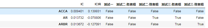
第三步,我们观测一下统计结果。EffectTestresult,下图未完全显示。
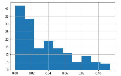
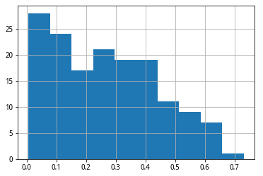
然后观察IC平均值,和ICIR的分布情况。
通过观察,我主观决定,筛选标准如下:
IC均值绝对值大于0.07,ICIR绝对值大于0.4,测试一,测试二-胜者组,测试三-胜者组,必须通过
测试二、测试三中要至少通过3个。
欢迎大家采用其他的筛选标准来最优化组合,在第二步的4中,也可以调整一下测试标准,4的检验结果存在变量effect_test_score_dict中。
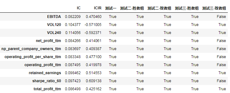
通过筛选,我们得到了如下因子:
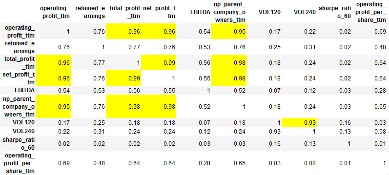
我们发现有很多因子非常相似,比如不同日期的vol,以及各种profit。所以我们需要剔除一些高度相关的因子。
如何计算因子的相关性呢。我们把股票对应因子数换成该股票所在的分组数。然后计算在同一时期,不同因子的股票分组序列的相关系数。由于我们有很多期,所以需要将这些相关系数矩阵取平均,得到的结果如下:
结合上面因子和测试结果,最后我剔除了['operating_profit_ttm','net_profit_ttm','np_parent_company_owners_ttm','VOL120'],这四个因子。因为IC,ICIR略差些,相比于同类因子。
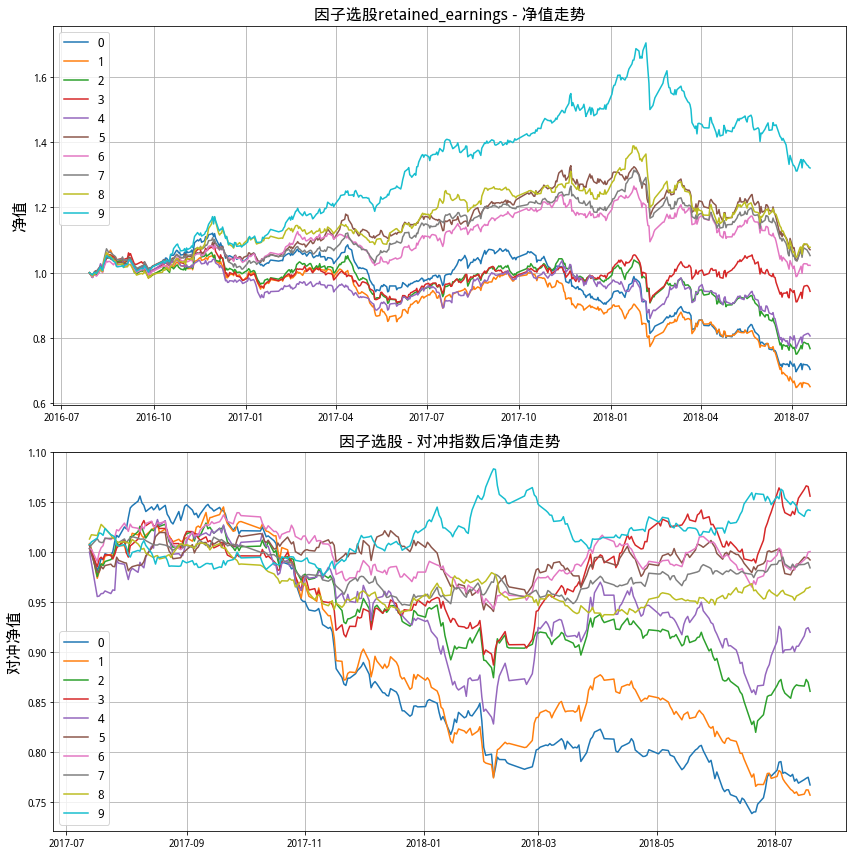
对于最后筛选出的因子,画出10分组的收益图,比如说:
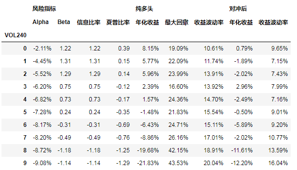
因子的分组组合统计,比如说:
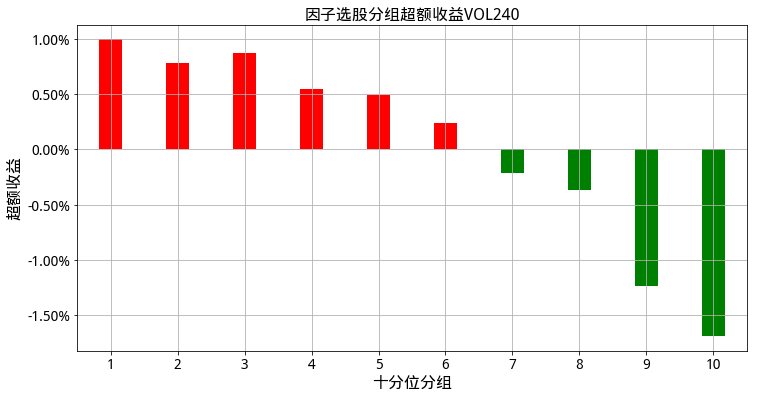
因子的超额收益图,比如说:
图看起来基本上都体面。
下一次,就是把这些有效因子带入回测模块了。Good Luck~!
大家多多交流,欢迎批评指正。
# Step I: 读取第一步因子生成的数据数据
import time
import datetime
import jqdata
import datetime
from multiprocessing.dummy import Pool as ThreadPool
from jqfactor import Factor,calc_factors
import pandas as pd
import statsmodels.api as sm
import scipy.stats as st
import pickle
pkl_file = open('MyPackage.pkl', 'rb')
load_Package = pickle.load(pkl_file)
g_univ_dict,return_df,all_return_df,raw_factor_dict,all_factor_dict,all_industry_df=load_Package

univ_dict=g_univ_dict

#factor_dict={}
#factor_dict['cfo_to_ev']=all_factor_dict['cfo_to_ev']
#all_factor_dict=factor_dict
# Step II: 因子筛选用到的函数
def ic_calculator(factor,return_df,univ_dict):
    ic_list=[]
    p_value_list=[]
    for date in list(univ_dict.keys()):   #这里是循环
        univ=univ_dict[date]
        univ=list(set(univ)&set(factor.loc[date].dropna().index)&set(return_df.loc[date].dropna().index))
        if len(univ)<10:
            continue
        factor_se=factor.loc[date,univ]
        return_se=return_df.loc[date,univ]
        ic,p_value=st.spearmanr(factor_se,return_se)
        ic_list.append(ic)
        p_value_list.append(p_value)
    return ic_list

# 1.回测基础数据计算
def all_Group_Return_calculator(factor,univ_dict,all_return_df,GroupNum=10):
    all_date_list=list(all_return_df.index)
    date_list=list(univ_dict.keys())
    all_Group_Ret_df=pd.DataFrame(index=all_date_list,columns=list(np.array(range(GroupNum))))
    for n in range(len(date_list)-1):
        start=date_list[n]
        end=date_list[n+1]
        univ=univ_dict[start]
        univ=set(univ)&set(factor.loc[start].dropna().index)
        factor_se_stock=list(factor.loc[start,univ].dropna().sort_values().index)
        N=len(factor_se_stock)
        for i in range(GroupNum):
            group_stock=factor_se_stock[int(N/GroupNum*i):int(N/GroupNum*(i+1))]
            # 下面两行是关键
            cumret=(all_return_df.loc[start:end,group_stock]+1).cumprod().mean(axis=1)
            all_Group_Ret_df.loc[start:end,i]=cumret.shift(1).fillna(1).pct_change().shift(-1)
            #(((all_return_df.loc[start:end,group_stock]+1).cumprod()-1).mean(axis=1)+1).pct_change().shift(-1)
    all_Group_Ret_df=all_Group_Ret_df[date_list[0]:].shift(1).fillna(0)
    return all_Group_Ret_df

def Group_Return_calculator(factor,univ_dict,return_df,GroupNum=10):
    GroupRet_df=pd.DataFrame(index=list(list(univ_dict.keys())),columns=list(np.array(range(GroupNum))))
    for date in list(univ_dict.keys()):    #这个也是个循环
        univ=univ_dict[date]
        univ=list(set(univ)&set(factor.loc[date].dropna().index)&set(return_df.loc[date].dropna().index))
        factor_se_stock=list(factor.loc[date,univ].sort_values().index)
        N=len(factor_se_stock)
        for i in range(GroupNum):
            group_stock=factor_se_stock[int(N/GroupNum*i):int(N/GroupNum*(i+1))]
            GroupRet_df.loc[date,i]=return_df.loc[date,group_stock].mean()
    return GroupRet_df.shift(1).fillna(0)

def get_index_return(univ_dict,index,count=250):
    trade_date_list=list(univ_dict.keys())
    date=max(trade_date_list)
    price=get_price(index,end_date=date,count=count,fields=['close'])['close']
    price_return=price.loc[trade_date_list[0]:].pct_change().fillna(0)
    price_return_by_tradeday=price.loc[trade_date_list].pct_change().fillna(0)
    return price_return,price_return_by_tradeday

def effect_test(univ_dict,key,group_return,group_excess_return):

    daylength=(list(univ_dict.keys())[-1]-list(univ_dict.keys())[0]).days
    annual_return=np.power(cumprod(group_return+1).iloc[-1,:],365/daylength)
    index_annual_return=np.power((index_return+1).cumprod().iloc[-1],365/daylength)

    # Test One: 组合序列与组合收益的相关性,相关性大于0.5
    sequence=pd.Series(np.array(range(10)))
    test_one_corr=annual_return.corr(sequence)
    test_one_passgrade=0.5
    test_one_pass=abs(test_one_corr)>test_one_passgrade

    if test_one_corr<0:
        wingroup,losegroup=0,9
    else:
        wingroup,losegroup=9,0

    # Test Two: 赢家组合明显跑赢市场,输家组合明显跑输市场,程度大于5%
    test_two_passgrade=0.05
    test_two_win_excess=annual_return[wingroup]-index_annual_return
    test_two_win_pass=test_two_win_excess>test_two_passgrade
    test_two_lose_excess=index_annual_return-annual_return[losegroup]
    test_two_lose_pass=test_two_lose_excess>test_two_passgrade
    test_two_pass=test_two_win_pass&test_two_lose_pass

    # Test Tree: 高收益组合跑赢基准的概率,低收益组合跑赢基准的概率,概率大小0.5
    test_three_grade=0.5
    test_three_win_prob=(group_excess_return[wingroup]>0).sum()/len(group_excess_return[wingroup])
    test_three_win_pass=test_three_win_prob>0.5
    test_three_lose_prob=(group_excess_return[losegroup]<0).sum()/len(group_excess_return[losegroup])
    test_three_lose_pass=test_three_lose_prob>0.5
    test_three_pass=test_three_win_pass&test_three_lose_pass

    test_result=[test_one_pass,test_two_win_pass,test_two_lose_pass,test_three_win_pass,test_three_lose_pass]
    test_score=[test_one_corr,test_two_win_excess,test_two_lose_excess,test_three_win_prob,test_three_lose_prob]

    return test_result,test_score
# 计算每个因子的评分和筛选结果

starttime=time.clock()

print('\n计算IC_IR:')
count=1
ic_list_dict={}
for key,factor in all_factor_dict.items():
    ic_list=ic_calculator(factor,return_df,univ_dict)
    ic_list_dict[key]=ic_list
    print(count,end=',')
    count=count+1
# 整理结果
ic_df=pd.DataFrame(ic_list_dict,index=list(univ_dict.keys())[:-1])
ic_ir_se=ic_df.mean()/ic_df.std()
ic_avg_se=ic_df.mean().abs()

print('\n计算分组收益:')
count=1
GroupNum=10
all_Factor_Group_Return_dict={}                    ##这个用于计算NAV,再筛选出因子之后再用更效率
Factor_Group_Return_dict={}
for key,factor in all_factor_dict.items():
# 全return
    all_GroupRet_df=all_Group_Return_calculator(factor,univ_dict,all_return_df,GroupNum)
    all_Factor_Group_Return_dict[key]=all_GroupRet_df
# 调仓期return
    GroupRet_df=Group_Return_calculator(factor,univ_dict,return_df,GroupNum)
    Factor_Group_Return_dict[key]=GroupRet_df
    print(count,end=',')
    count=count+1

print('\n计算指数收益:')
count=1
index='000300.XSHG'
index_return,index_return_by_tradeday=get_index_return(univ_dict,index)
Factor_Group_Excess_Return_dict={}
for key,group_return in Factor_Group_Return_dict.items():
    Factor_Group_Excess_Return_dict[key]=group_return.subtract(index_return_by_tradeday,axis=0)
    print(count,end=',')
    count=count+1

print('\n因子有效性测试:')
count=1
effect_test_result_dict={}
effect_test_score_dict={}
for key,group_return in Factor_Group_Return_dict.items():
    group_excess_return=Factor_Group_Excess_Return_dict[key]
    effect_test_result_dict[key],effect_test_score_dict[key]=effect_test(univ_dict,key,group_return,group_excess_return)
    print(count,end=',')
    count=count+1

print('\npickle序列化')
Package_ET=[ic_avg_se,ic_ir_se,effect_test_result_dict,effect_test_score_dict,\
           all_Factor_Group_Return_dict,Factor_Group_Return_dict,index_return,index_return_by_tradeday,\
           Factor_Group_Excess_Return_dict]
pkl_file = open('MyPackage_ET.pkl', 'wb')
pickle.dump(Package_ET,pkl_file,0)
pkl_file.close()

endtime=time.clock()
runtime=endtime-starttime
print('因子测试运行完成,用时 %.2f 秒' % runtime)
# 读取因子
import pickle
pkl_file = open('MyPackage_ET.pkl', 'rb')
load_Package = pickle.load(pkl_file)
ic_avg_se,ic_ir_se,effect_test_result_dict,effect_test_score_dict,\
all_Factor_Group_Return_dict,Factor_Group_Return_dict,index_return,index_return_by_tradeday,\
Factor_Group_Excess_Return_dict=load_Package
EffectTestresult=pd.concat([ic_avg_se.to_frame('a'),ic_ir_se.to_frame('b'),pd.DataFrame(effect_test_result_dict).T],axis=1)
columns=['IC','ICIR','测试一', '测试二-胜者组', '测试二-败者组', '测试三-胜者组', '测试三-败者组']
EffectTestresult.columns=columns
EffectTestresult2=pd.concat([ic_avg_se.to_frame('a'),ic_ir_se.to_frame('b'),pd.DataFrame(effect_test_score_dict).T],axis=1)
columns=['IC','ICIR','测试一', '测试二-胜者组', '测试二-败者组', '测试三-胜者组', '测试三-败者组']
EffectTestresult2.columns=columns
EffectTestresult
EffectTestresult['IC'].sort_values(ascending=False).hist()

EffectTestresult['ICIR'].abs().sort_values(ascending=False).hist()

#筛选有效因子
# IC大于0.07,ICIR大于0.4,测试一,测试二-胜者组,测试三-胜者组,必须通过
# 测试二、测试三中要至少通过3个。
index_ic=EffectTestresult['IC']>0.07
index_icir=EffectTestresult['ICIR'].abs()>0.4
test_index=all(EffectTestresult.iloc[:,[2,3,5]],axis=1)
test2_index=sum(EffectTestresult.iloc[:,3:6],axis=1)>=3
filter_index=index_ic&index_icir&test_index&test2_index
EffectFactorresult=EffectTestresult.loc[filter_index,:]
# 生成有效因子字典
EffectFactor=list(EffectFactorresult.index)
Effect_factor_dict={key:value for key,value in all_factor_dict.items() if key in EffectFactor}
EffectFactorresult
def Group_Score_calculator(factor,univ_dict,signal,GroupNum=20):

    Score_df=pd.DataFrame(index=list(factor.index),columns=list(factor.columns))

    for date in list(univ_dict.keys()):    #这个也是个循环
        univ=univ_dict[date]
        univ=list(set(univ)&set(factor.loc[date].dropna().index))
        factor_se_stock=list(factor.loc[date,univ].sort_values().index)
        N=len(factor_se_stock)
        for i in range(GroupNum):
            group_stock=factor_se_stock[int(N/GroupNum*i):int(N/GroupNum*(i+1))]
            if signal=='ascending':
                Score_df.loc[date,group_stock]=i
            else:
                Score_df.loc[date,group_stock]=GroupNum-i

    return Score_df

# 计算相关性矩阵
def factor_corr_calculator(Group_Score_Dict,univ_dict):

    Group_Score_dict_by_day={}
    Group_Score_Corr_dict_by_day={}

    # 每日的因子序列
    for Date in list(univ_dict.keys()):
        Group_Score_df=pd.DataFrame()
        univ=univ_dict[Date]
        for Factor in list(Group_Score_dict.keys()):
            Group_Score_df=Group_Score_df.append(Group_Score_dict[Factor].loc[Date,univ].to_frame(Factor).T)
        Group_Score_dict_by_day[Date]=Group_Score_df.T.fillna(4.5)
        Group_Score_Corr_dict_by_day[Date]=Group_Score_dict_by_day[Date].corr()

    # 算平均数
    N=len(list(univ_dict.keys()))
    Group_Score_Corr=Group_Score_Corr_dict_by_day[list(univ_dict.keys())[0]]
    for Date in list(univ_dict.keys())[1:]:
        Group_Score_Corr=Group_Score_Corr+Group_Score_Corr_dict_by_day[Date]

    return (Group_Score_Corr/N).round(2)

# 给因子赋值
Group_Score_dict={}
for key,factor in Effect_factor_dict.items():
    signal='ascending' if ic_ir_se[key]>0 else 'descending'
    Group_Score_dict[key]=Group_Score_calculator(factor,univ_dict,signal,20)

# 计算因子相关系数
factor_corrmatrix=factor_corr_calculator(Group_Score_dict,univ_dict)
factor_corrmatrix
# 比较后去掉一些因子
# operating_profit_ttm,net_profit_ttm,np_parent_company_owners_ttm,VOL120
removed_factor=['operating_profit_ttm','net_profit_ttm','np_parent_company_owners_ttm','VOL120']
Effect_factor_dict={key:value for key,value in Effect_factor_dict.items() if key not in removed_factor}
def plot_nav(all_return_df,index_return,key):
# Preallocate figures
    fig = plt.figure(figsize=(12,12))
    fig.set_facecolor('white')
    fig.set_tight_layout(True)
    ax1 = fig.add_subplot(211)
    ax2 = fig.add_subplot(212)
    ax1.grid()
    ax2.grid()
    ax1.set_ylabel(u"净值", fontsize=16)
    ax2.set_ylabel(u"对冲净值", fontsize=16)
    ax1.set_title(u"因子选股{} - 净值走势".format(key),fontsize=16)
    ax2.set_title(u"因子选股 - 对冲指数后净值走势", fontsize=16)
# preallocate data
    date=list(all_return_df.index)
    sequence=all_return_df.columns
# plot nav
    for sq in sequence:
        nav=(1+all_return_df[sq]).cumprod()
        nav_excess=(1+all_return_df[sq]-index_return).cumprod()
        ax1.plot(date,nav,label=str(sq))
        ax2.plot(date,nav_excess,label=str(sq))
    ax1.legend(loc=0,fontsize=12)
    ax2.legend(loc=0,fontsize=12)

def polish(x):
    return '%.2f%%' % (x*100)

def result_stats(key,all_return_df,index_return):

    # Preallocate result DataFrame
    sequences=all_return_df.columns

    cols = [(u'风险指标', u'Alpha'), (u'风险指标', u'Beta'), (u'风险指标', u'信息比率'), (u'风险指标', u'夏普比率'),
            (u'纯多头', u'年化收益'), (u'纯多头', u'最大回撤'), (u'纯多头', u'收益波动率'),
            (u'对冲后', u'年化收益'), (u'对冲后', u'收益波动率')]
    columns = pd.MultiIndex.from_tuples(cols)
    result_df = pd.DataFrame(index = sequences,columns=columns)
    result_df.index.name = "%s" % (key)

    for sq in sequences:  #循环在这里开始

        # 净值
        return_data=all_return_df[sq]
        return_data_excess=return_data-index_return
        nav=(1+return_data).cumprod()
        nav_excess=(1+return_data_excess).cumprod()
        nav_index=(1+index_return).cumprod()

        # Beta
        beta=return_data.corr(index_return)*return_data.std()/index_return.std()
        beta_excess=return_data_excess.corr(index_return)*return_data_excess.std()/index_return.std()

        #年化收益
        daylength=(return_data.index[-1]-return_data.index[0]).days
        yearly_return=np.power(nav.iloc[-1],1.0*365/daylength)-1
        yearly_return_excess=np.power(nav_excess.iloc[-1],1.0*365/daylength)-1
        yearly_index_return=np.power(nav_index.iloc[-1],1.0*365/daylength)-1

        # 最大回撤 其实这个完全看不懂
        max_drawdown=max([1-v/max(1,max(nav.iloc[:i+1])) for i,v in enumerate(nav)])
        #max_drawdown_excess=max([1-v/max(1,max(nav_excess.iloc[:i+1])) for i,v in enumerate(nav_excess)])

        # 波动率
        vol=return_data.std()*sqrt(252)
        vol_excess=return_data_excess.std()*sqrt(252)

        # Alpha
        rf=0.04
        alpha=yearly_return-(rf+beta*(yearly_return-yearly_index_return))
        alpha_excess=yearly_return_excess-(rf+beta_excess*(yearly_return-yearly_index_return))

        # 信息比率
        ir=(yearly_return-yearly_index_return)/(return_data_excess.std()*sqrt(252))

        # 夏普比率
        sharpe=(yearly_return-rf)/vol

        # 美化打印

        alpha,yearly_return,max_drawdown,vol,yearly_return_excess,vol_excess=\
        map(polish,[alpha,yearly_return,max_drawdown,vol,yearly_return_excess,vol_excess])
        sharpe=round(sharpe,2)
        ir=round(ir,2)
        beta=round(ir,2)

        result_df.loc[sq]=[alpha,beta,ir,sharpe,yearly_return,max_drawdown,vol,yearly_return_excess,vol_excess]
    return result_df

def draw_excess_return(excess_return,key):
    excess_return_mean=excess_return[1:].mean()
    excess_return_mean.index = map(lambda x:int(x)+1,excess_return_mean.index)
    excess_plus=excess_return_mean[excess_return_mean>0]
    excess_minus=excess_return_mean[excess_return_mean<0]

    fig = plt.figure(figsize=(12, 6))
    fig.set_facecolor('white')
    ax1 = fig.add_subplot(111)
    ax1.bar(excess_plus.index, excess_plus.values, align='center', color='r', width=0.35)
    ax1.bar(excess_minus.index, excess_minus.values, align='center', color='g', width=0.35)
    ax1.set_xlim(left=0.5, right=len(excess_return_mean)+0.5)
    ax1.set_ylabel(u'超额收益', fontsize=16)
    ax1.set_xlabel(u'十分位分组', fontsize=16)
    ax1.set_xticks(excess_return_mean.index)
    ax1.set_xticklabels([int(x) for x in ax1.get_xticks()], fontsize=14)
    ax1.set_yticklabels([str(x*100)+'0%' for x in ax1.get_yticks()], fontsize=14)
    ax1.set_title(u"因子选股分组超额收益{}".format(key), fontsize=16)
    ax1.grid()
for key in list(Effect_factor_dict.keys()):
    plot_nav(all_Factor_Group_Return_dict[key],index_return,key)


result_dict={}
for key in list(Effect_factor_dict.keys()):
    result_df=result_stats(key,all_Factor_Group_Return_dict[key],index_return)
    result_dict[key]=result_df
    print(result_df)
result_dict['VOL240']
for key in list(Effect_factor_dict.keys()):
    draw_excess_return(Factor_Group_Excess_Return_dict[key],key)