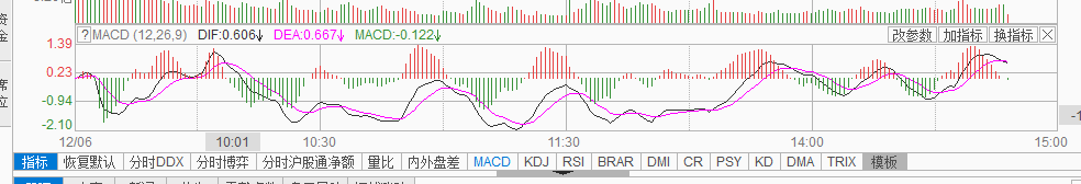
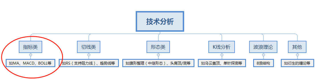
说到技术指标,想必不论新韭老韭都能随口念出几个来,是判断行情走势的衍生工具,也是行情软件中必备的板块内容,技术分析一直在大多数股民中备受好评,各个频道的股评专家也是乐此不疲。
股市参与者千万人,在同一市场中博弈,作为个人投资者获取行业或公司信息并无优势,然而关于市场所有的信息最终都会落到交易上,会体现在成交量和价格上,量价信息这个层面来讲,市场是公平的,这也是技术分析能够为大多数人使用的原因之一。
使用技术分析之前,我们需要了解到,所有技术分析能够成立,是建立在以下的三大基石之上
[(0, 'None'),(1, 'MA'),(2, 'MA1'),(3, 'EMA'),(4, 'EMA1'),(5, 'MACD'),(6, 'KDJ'),(7, 'CCI'),(8, 'RSI'),(9, 'BOLL'),(10, 'BIAS'),(11, 'TRIX'),(12, 'BBI'),(13, 'PSY')]
下面是指标在沪深300指数上的择时表现,以按收益进行排序
['10','11','12','13','14','15','16','17','18','19','20','21','22','23','24','25','26','27','28','30']
通过上述的测试结果,我们初步发现如下的情况
本篇为了避免个别标的自身特性的影响,都是拿指数进行的测试,然而不同指数本身也有各自的特点,可以借助已有的代码进行更多标的枚举暴力测试,通过多回测方法进一步挖掘更为有效的指标参数。
20181225:感谢@宋一堆 的改进思路,已将可用做空版代码附在评论区
20181225:感谢评论区sailer 和 iamrobot 的留言,文章统计结果已替换为修正后的结果,代码已更改附在评论区
#1 先导入所需要的程序包
import datetime
import numpy as np
import pandas as pd
import time
from jqdata import *
from pandas import Series, DataFrame
import matplotlib.pyplot as plt
import seaborn as sns
import itertools
import copy
import pickle
# 定义类'参数分析'
class parameter_analysis(object):
# 定义函数中不同的变量
def __init__(self, algorithm_id=None):
self.algorithm_id = algorithm_id # 回测id
self.params_df = pd.DataFrame() # 回测中所有调参备选值的内容,列名字为对应修改面两名称,对应回测中的 g.XXXX
self.results = {} # 回测结果的回报率,key 为 params_df 的行序号,value 为
self.evaluations = {} # 回测结果的各项指标,key 为 params_df 的行序号,value 为一个 dataframe
self.backtest_ids = {} # 回测结果的 id
# 新加入的基准的回测结果 id,可以默认为空 '',则使用回测中设定的基准
self.benchmark_id = None
self.benchmark_returns = [] # 新加入的基准的回测回报率
self.returns = {} # 记录所有回报率
self.excess_returns = {} # 记录超额收益率
self.log_returns = {} # 记录收益率的 log 值
self.log_excess_returns = {} # 记录超额收益的 log 值
self.dates = [] # 回测对应的所有日期
self.excess_max_drawdown = {} # 计算超额收益的最大回撤
self.excess_annual_return = {} # 计算超额收益率的年化指标
self.evaluations_df = pd.DataFrame() # 记录各项回测指标,除日回报率外
# 定义排队运行多参数回测函数
def run_backtest(self, #
algorithm_id=None, # 回测策略id
running_max=10, # 回测中同时巡行最大回测数量
start_date='2006-01-01', # 回测的起始日期
end_date='2016-11-30', # 回测的结束日期
frequency='day', # 回测的运行频率
initial_cash='1000000', # 回测的初始持仓金额
param_names=[], # 回测中调整参数涉及的变量
param_values=[] # 回测中每个变量的备选参数值
):
# 当此处回测策略的 id 没有给出时,调用类输入的策略 id
if algorithm_id == None: algorithm_id=self.algorithm_id
# 生成所有参数组合并加载到 df 中
# 包含了不同参数具体备选值的排列组合中一组参数的 tuple 的 list
param_combinations = list(itertools.product(*param_values))
# 生成一个 dataframe, 对应的列为每个调参的变量,每个值为调参对应的备选值
to_run_df = pd.DataFrame(param_combinations)
# 修改列名称为调参变量的名字
to_run_df.columns = param_names
# 设定运行起始时间和保存格式
start = time.time()
# 记录结束的运行回测
finished_backtests = {}
# 记录运行中的回测
running_backtests = {}
# 计数器
pointer = 0
# 总运行回测数目,等于排列组合中的元素个数
total_backtest_num = len(param_combinations)
# 记录回测结果的回报率
all_results = {}
# 记录回测结果的各项指标
all_evaluations = {}
# 在运行开始时显示
print ('【已完成|运行中|待运行】:'),
# 当运行回测开始后,如果没有全部运行完全的话:
while len(finished_backtests)<total_backtest_num:
# 显示运行、完成和待运行的回测个数
print('[%s|%s|%s].' % (len(finished_backtests),
len(running_backtests),
(total_backtest_num-len(finished_backtests)-len(running_backtests)) )),
# 记录当前运行中的空位数量
to_run = min(running_max-len(running_backtests), total_backtest_num-len(running_backtests)-len(finished_backtests))
# 把可用的空位进行跑回测
for i in range(pointer, pointer+to_run):
# 备选的参数排列组合的 df 中第 i 行变成 dict,每个 key 为列名字,value 为 df 中对应的值
params = to_run_df.iloc[i].to_dict()
# 记录策略回测结果的 id,调整参数 extras 使用 params 的内容
backtest = create_backtest(algorithm_id = algorithm_id,
start_date = start_date,
end_date = end_date,
frequency = frequency,
initial_cash = initial_cash,
extras = params,
# 再回测中把改参数的结果起一个名字,包含了所有涉及的变量参数值
name = str(params)
)
# 记录运行中 i 回测的回测 id
running_backtests[i] = backtest
# 计数器计数运行完的数量
pointer = pointer+to_run
# 获取回测结果
failed = []
finished = []
# 对于运行中的回测,key 为 to_run_df 中所有排列组合中的序数
for key in running_backtests.keys():
# 研究调用回测的结果,running_backtests[key] 为运行中保存的结果 id
bt = get_backtest(running_backtests[key])
# 获得运行回测结果的状态,成功和失败都需要运行结束后返回,如果没有返回则运行没有结束
status = bt.get_status()
# 当运行回测失败
if status == 'failed':
# 失败 list 中记录对应的回测结果 id
failed.append(key)
# 当运行回测成功时
elif status == 'done':
# 成功 list 记录对应的回测结果 id,finish 仅记录运行成功的
finished.append(key)
# 回测回报率记录对应回测的回报率 dict, key to_run_df 中所有排列组合中的序数, value 为回报率的 dict
# 每个 value 一个 list 每个对象为一个包含时间、日回报率和基准回报率的 dict
all_results[key] = bt.get_results()
# 回测回报率记录对应回测结果指标 dict, key to_run_df 中所有排列组合中的序数, value 为回测结果指标的 dataframe
all_evaluations[key] = bt.get_risk()
# 记录运行中回测结果 id 的 list 中删除失败的运行
for key in failed:
running_backtests.pop(key)
# 在结束回测结果 dict 中记录运行成功的回测结果 id,同时在运行中的记录中删除该回测
for key in finished:
finished_backtests[key] = running_backtests.pop(key)
# 当一组同时运行的回测结束时报告时间
if len(finished_backtests) != 0 and len(finished_backtests) % running_max == 0 and to_run !=0:
# 记录当时时间
middle = time.time()
# 计算剩余时间,假设没工作量时间相等的话
remain_time = (middle - start) * (total_backtest_num - len(finished_backtests)) / len(finished_backtests)
# print 当前运行时间
print('[已用%s时,尚余%s时,请不要关闭浏览器].' % (str(round((middle - start) / 60.0 / 60.0,3)),
str(round(remain_time / 60.0 / 60.0,3)))),
# 5秒钟后再跑一下
time.sleep(30)
# 记录结束时间
end = time.time()
print ('')
print('【回测完成】总用时:%s秒(即%s小时)。' % (str(int(end-start)),
str(round((end-start)/60.0/60.0,2)))),
# 对应修改类内部对应
self.params_df = to_run_df
self.results = all_results
self.evaluations = all_evaluations
self.backtest_ids = finished_backtests
#7 最大回撤计算方法
def find_max_drawdown(self, returns):
# 定义最大回撤的变量
result = 0
# 记录最高的回报率点
historical_return = 0
# 遍历所有日期
for i in range(len(returns)):
# 最高回报率记录
historical_return = max(historical_return, returns[i])
# 最大回撤记录
drawdown = 1-(returns[i] + 1) / (historical_return + 1)
# 记录最大回撤
result = max(drawdown, result)
# 返回最大回撤值
return result
# log 收益、新基准下超额收益和相对与新基准的最大回撤
def organize_backtest_results(self, benchmark_id=None):
# 若新基准的回测结果 id 没给出
if benchmark_id==None:
# 使用默认的基准回报率,默认的基准在回测策略中设定
self.benchmark_returns = [x['benchmark_returns'] for x in self.results[0]]
# 当新基准指标给出后
else:
# 基准使用新加入的基准回测结果
self.benchmark_returns = [x['returns'] for x in get_backtest(benchmark_id).get_results()]
# 回测日期为结果中记录的第一项对应的日期
self.dates = [x['time'] for x in self.results[0]]
# 对应每个回测在所有备选回测中的顺序 (key),生成新数据
# 由 {key:{u'benchmark_returns': 0.022480100091729405,
# u'returns': 0.03184566700000002,
# u'time': u'2006-02-14'}} 格式转化为:
# {key: []} 格式,其中 list 为对应 date 的一个回报率 list
for key in self.results.keys():
self.returns[key] = [x['returns'] for x in self.results[key]]
# 生成对于基准(或新基准)的超额收益率
for key in self.results.keys():
self.excess_returns[key] = [(x+1)/(y+1)-1 for (x,y) in zip(self.returns[key], self.benchmark_returns)]
# 生成 log 形式的收益率
for key in self.results.keys():
self.log_returns[key] = [log(x+1) for x in self.returns[key]]
# 生成超额收益率的 log 形式
for key in self.results.keys():
self.log_excess_returns[key] = [log(x+1) for x in self.excess_returns[key]]
# 生成超额收益率的最大回撤
for key in self.results.keys():
self.excess_max_drawdown[key] = self.find_max_drawdown(self.excess_returns[key])
# 生成年化超额收益率
for key in self.results.keys():
self.excess_annual_return[key] = (self.excess_returns[key][-1]+1)**(252./float(len(self.dates)))-1
# 把调参数据中的参数组合 df 与对应结果的 df 进行合并
self.evaluations_df = pd.concat([self.params_df, pd.DataFrame(self.evaluations).T], axis=1)
# self.evaluations_df =
# 获取最总分析数据,调用排队回测函数和数据整理的函数
def get_backtest_data(self,
algorithm_id=None, # 回测策略id
benchmark_id=None, # 新基准回测结果id
file_name='results.pkl', # 保存结果的 pickle 文件名字
running_max=10, # 最大同时运行回测数量
start_date='2006-01-01', # 回测开始时间
end_date='2016-11-30', # 回测结束日期
frequency='day', # 回测的运行频率
initial_cash='1000000', # 回测初始持仓资金
param_names=[], # 回测需要测试的变量
param_values=[] # 对应每个变量的备选参数
):
# 调运排队回测函数,传递对应参数
self.run_backtest(algorithm_id=algorithm_id,
running_max=running_max,
start_date=start_date,
end_date=end_date,
frequency=frequency,
initial_cash=initial_cash,
param_names=param_names,
param_values=param_values
)
# 回测结果指标中加入 log 收益率和超额收益率等指标
self.organize_backtest_results(benchmark_id)
# 生成 dict 保存所有结果。
results = {'returns':self.returns,
'excess_returns':self.excess_returns,
'log_returns':self.log_returns,
'log_excess_returns':self.log_excess_returns,
'dates':self.dates,
'benchmark_returns':self.benchmark_returns,
'evaluations':self.evaluations,
'params_df':self.params_df,
'backtest_ids':self.backtest_ids,
'excess_max_drawdown':self.excess_max_drawdown,
'excess_annual_return':self.excess_annual_return,
'evaluations_df':self.evaluations_df}
# 保存 pickle 文件
pickle_file = open(file_name, 'wb')
pickle.dump(results, pickle_file)
pickle_file.close()
# 读取保存的 pickle 文件,赋予类中的对象名对应的保存内容
def read_backtest_data(self, file_name='results.pkl'):
pickle_file = open(file_name, 'rb')
results = pickle.load(pickle_file)
self.returns = results['returns']
self.excess_returns = results['excess_returns']
self.log_returns = results['log_returns']
self.log_excess_returns = results['log_excess_returns']
self.dates = results['dates']
self.benchmark_returns = results['benchmark_returns']
self.evaluations = results['evaluations']
self.params_df = results['params_df']
self.backtest_ids = results['backtest_ids']
self.excess_max_drawdown = results['excess_max_drawdown']
self.excess_annual_return = results['excess_annual_return']
self.evaluations_df = results['evaluations_df']
# 回报率折线图
def plot_returns(self):
# 通过figsize参数可以指定绘图对象的宽度和高度,单位为英寸;
fig = plt.figure(figsize=(20,8))
ax = fig.add_subplot(111)
# 作图
for key in self.returns.keys():
ax.plot(range(len(self.returns[key])), self.returns[key], label=key)
# 设定benchmark曲线并标记
ax.plot(range(len(self.benchmark_returns)), self.benchmark_returns, label='benchmark', c='k', linestyle='--')
ticks = [int(x) for x in np.linspace(0, len(self.dates)-1, 11)]
plt.xticks(ticks, [self.dates[i] for i in ticks])
# 设置图例样式
ax.legend(loc = 2, fontsize = 10)
# 设置y标签样式
ax.set_ylabel('returns',fontsize=20)
# 设置x标签样式
ax.set_yticklabels([str(x*100)+'% 'for x in ax.get_yticks()])
# 设置图片标题样式
ax.set_title("Strategy's performances with different parameters", fontsize=21)
plt.xlim(0, len(self.returns[0]))
# 超额收益率图
def plot_excess_returns(self):
# 通过figsize参数可以指定绘图对象的宽度和高度,单位为英寸;
fig = plt.figure(figsize=(20,8))
ax = fig.add_subplot(111)
# 作图
for key in self.returns.keys():
ax.plot(range(len(self.excess_returns[key])), self.excess_returns[key], label=key)
# 设定benchmark曲线并标记
ax.plot(range(len(self.benchmark_returns)), [0]*len(self.benchmark_returns), label='benchmark', c='k', linestyle='--')
ticks = [int(x) for x in np.linspace(0, len(self.dates)-1, 11)]
plt.xticks(ticks, [self.dates[i] for i in ticks])
# 设置图例样式
ax.legend(loc = 2, fontsize = 10)
# 设置y标签样式
ax.set_ylabel('excess returns',fontsize=20)
# 设置x标签样式
ax.set_yticklabels([str(x*100)+'% 'for x in ax.get_yticks()])
# 设置图片标题样式
ax.set_title("Strategy's performances with different parameters", fontsize=21)
plt.xlim(0, len(self.excess_returns[0]))
# log回报率图
def plot_log_returns(self):
# 通过figsize参数可以指定绘图对象的宽度和高度,单位为英寸;
fig = plt.figure(figsize=(20,8))
ax = fig.add_subplot(111)
# 作图
for key in self.returns.keys():
ax.plot(range(len(self.log_returns[key])), self.log_returns[key], label=key)
# 设定benchmark曲线并标记
ax.plot(range(len(self.benchmark_returns)), [log(x+1) for x in self.benchmark_returns], label='benchmark', c='k', linestyle='--')
ticks = [int(x) for x in np.linspace(0, len(self.dates)-1, 11)]
plt.xticks(ticks, [self.dates[i] for i in ticks])
# 设置图例样式
ax.legend(loc = 2, fontsize = 10)
# 设置y标签样式
ax.set_ylabel('log returns',fontsize=20)
# 设置图片标题样式
ax.set_title("Strategy's performances with different parameters", fontsize=21)
plt.xlim(0, len(self.log_returns[0]))
# 超额收益率的 log 图
def plot_log_excess_returns(self):
# 通过figsize参数可以指定绘图对象的宽度和高度,单位为英寸;
fig = plt.figure(figsize=(20,8))
ax = fig.add_subplot(111)
# 作图
for key in self.returns.keys():
ax.plot(range(len(self.log_excess_returns[key])), self.log_excess_returns[key], label=key)
# 设定benchmark曲线并标记
ax.plot(range(len(self.benchmark_returns)), [0]*len(self.benchmark_returns), label='benchmark', c='k', linestyle='--')
ticks = [int(x) for x in np.linspace(0, len(self.dates)-1, 11)]
plt.xticks(ticks, [self.dates[i] for i in ticks])
# 设置图例样式
ax.legend(loc = 2, fontsize = 10)
# 设置y标签样式
ax.set_ylabel('log excess returns',fontsize=20)
# 设置图片标题样式
ax.set_title("Strategy's performances with different parameters", fontsize=21)
plt.xlim(0, len(self.log_excess_returns[0]))
# 回测的4个主要指标,包括总回报率、最大回撤夏普率和波动
def get_eval4_bar(self, sort_by=[]):
sorted_params = self.params_df
for by in sort_by:
sorted_params = sorted_params.sort(by)
indices = sorted_params.index
fig = plt.figure(figsize=(20,7))
# 定义位置
ax1 = fig.add_subplot(221)
# 设定横轴为对应分位,纵轴为对应指标
ax1.bar(range(len(indices)),
[self.evaluations[x]['algorithm_return'] for x in indices], 0.6, label = 'Algorithm_return')
plt.xticks([x+0.3 for x in range(len(indices))], indices)
# 设置图例样式
ax1.legend(loc='best',fontsize=15)
# 设置y标签样式
ax1.set_ylabel('Algorithm_return', fontsize=15)
# 设置y标签样式
ax1.set_yticklabels([str(x*100)+'% 'for x in ax1.get_yticks()])
# 设置图片标题样式
ax1.set_title("Strategy's of Algorithm_return performances of different quantile", fontsize=15)
# x轴范围
plt.xlim(0, len(indices))
# 定义位置
ax2 = fig.add_subplot(224)
# 设定横轴为对应分位,纵轴为对应指标
ax2.bar(range(len(indices)),
[self.evaluations[x]['max_drawdown'] for x in indices], 0.6, label = 'Max_drawdown')
plt.xticks([x+0.3 for x in range(len(indices))], indices)
# 设置图例样式
ax2.legend(loc='best',fontsize=15)
# 设置y标签样式
ax2.set_ylabel('Max_drawdown', fontsize=15)
# 设置x标签样式
ax2.set_yticklabels([str(x*100)+'% 'for x in ax2.get_yticks()])
# 设置图片标题样式
ax2.set_title("Strategy's of Max_drawdown performances of different quantile", fontsize=15)
# x轴范围
plt.xlim(0, len(indices))
# 定义位置
ax3 = fig.add_subplot(223)
# 设定横轴为对应分位,纵轴为对应指标
ax3.bar(range(len(indices)),
[self.evaluations[x]['sharpe'] for x in indices], 0.6, label = 'Sharpe')
plt.xticks([x+0.3 for x in range(len(indices))], indices)
# 设置图例样式
ax3.legend(loc='best',fontsize=15)
# 设置y标签样式
ax3.set_ylabel('Sharpe', fontsize=15)
# 设置x标签样式
ax3.set_yticklabels([str(x*100)+'% 'for x in ax3.get_yticks()])
# 设置图片标题样式
ax3.set_title("Strategy's of Sharpe performances of different quantile", fontsize=15)
# x轴范围
plt.xlim(0, len(indices))
# 定义位置
ax4 = fig.add_subplot(222)
# 设定横轴为对应分位,纵轴为对应指标
ax4.bar(range(len(indices)),
[self.evaluations[x]['algorithm_volatility'] for x in indices], 0.6, label = 'Algorithm_volatility')
plt.xticks([x+0.3 for x in range(len(indices))], indices)
# 设置图例样式
ax4.legend(loc='best',fontsize=15)
# 设置y标签样式
ax4.set_ylabel('Algorithm_volatility', fontsize=15)
# 设置x标签样式
ax4.set_yticklabels([str(x*100)+'% 'for x in ax4.get_yticks()])
# 设置图片标题样式
ax4.set_title("Strategy's of Algorithm_volatility performances of different quantile", fontsize=15)
# x轴范围
plt.xlim(0, len(indices))
#14 年化回报和最大回撤,正负双色表示
def get_eval(self, sort_by=[]):
sorted_params = self.params_df
for by in sort_by:
sorted_params = sorted_params.sort(by)
indices = sorted_params.index
# 大小
fig = plt.figure(figsize = (20, 8))
# 图1位置
ax = fig.add_subplot(111)
# 生成图超额收益率的最大回撤
ax.bar([x+0.3 for x in range(len(indices))],
[-self.evaluations[x]['max_drawdown'] for x in indices], color = '#32CD32',
width = 0.6, label = 'Max_drawdown', zorder=10)
# 图年化超额收益
ax.bar([x for x in range(len(indices))],
[self.evaluations[x]['annual_algo_return'] for x in indices], color = 'r',
width = 0.6, label = 'Annual_return')
plt.xticks([x+0.3 for x in range(len(indices))], indices)
# 设置图例样式
ax.legend(loc='best',fontsize=15)
# 基准线
plt.plot([0, len(indices)], [0, 0], c='k',
linestyle='--', label='zero')
# 设置图例样式
ax.legend(loc='best',fontsize=15)
# 设置y标签样式
ax.set_ylabel('Max_drawdown', fontsize=15)
# 设置x标签样式
ax.set_yticklabels([str(x*100)+'% 'for x in ax.get_yticks()])
# 设置图片标题样式
ax.set_title("Strategy's performances of different quantile", fontsize=15)
# 设定x轴长度
plt.xlim(0, len(indices))
#14 超额收益的年化回报和最大回撤
# 加入新的benchmark后超额收益和
def get_excess_eval(self, sort_by=[]):
sorted_params = self.params_df
for by in sort_by:
sorted_params = sorted_params.sort(by)
indices = sorted_params.index
# 大小
fig = plt.figure(figsize = (20, 8))
# 图1位置
ax = fig.add_subplot(111)
# 生成图超额收益率的最大回撤
ax.bar([x+0.3 for x in range(len(indices))],
[-self.excess_max_drawdown[x] for x in indices], color = '#32CD32',
width = 0.6, label = 'Excess_max_drawdown')
# 图年化超额收益
ax.bar([x for x in range(len(indices))],
[self.excess_annual_return[x] for x in indices], color = 'r',
width = 0.6, label = 'Excess_annual_return')
plt.xticks([x+0.3 for x in range(len(indices))], indices)
# 设置图例样式
ax.legend(loc='best',fontsize=15)
# 基准线
plt.plot([0, len(indices)], [0, 0], c='k',
linestyle='--', label='zero')
# 设置图例样式
ax.legend(loc='best',fontsize=15)
# 设置y标签样式
ax.set_ylabel('Max_drawdown', fontsize=15)
# 设置x标签样式
ax.set_yticklabels([str(x*100)+'% 'for x in ax.get_yticks()])
# 设置图片标题样式
ax.set_title("Strategy's performances of different quantile", fontsize=15)
# 设定x轴长度
plt.xlim(0, len(indices))
#2 设定回测策略 id
# 注意!注意!注意!这里的id是在 我的策略里面的编译运行的algorithmId,在浏览器地址里面复制一下
pa = parameter_analysis('5473a8b9e878d36100307a7d1c0405ee')
#3 运行回测
pa.get_backtest_data(file_name = 'results1.pkl',
                          running_max = 10,
                          benchmark_id = None,
                          start_date = '2008-12-05',
                           end_date = '2018-12-05',
                          frequency = 'day',
                          initial_cash = '100000000',
                          param_names = ['tech'],
                          param_values = [['None','MA','MA1','EMA','EMA1','MACD','KDJ','CCI','RSI','BOLL','BIAS','TRIX','BBI','PSY']]
                          )
【已完成|运行中|待运行】: [0|0|14]. [0|10|4]. [0|10|4]. [8|2|4]. [已用0.031时,尚余0.012时,请不要关闭浏览器]. [10|4|0]. [10|4|0].
【回测完成】总用时:206秒(即0.06小时)。
#4 数据读取
pa.read_backtest_data('results1.pkl')
#5 查看回测参数的df
pa.params_df
| tech | |
|---|---|
| 0 | None |
| 1 | MA |
| 2 | MA1 |
| 3 | EMA |
| 4 | EMA1 |
| 5 | MACD |
| 6 | KDJ |
| 7 | CCI |
| 8 | RSI |
| 9 | BOLL |
| 10 | BIAS |
| 11 | TRIX |
| 12 | BBI |
| 13 | PSY |
#6 查看回测结果指标
df = pa.evaluations_df
df
| tech | __version | algorithm_return | algorithm_volatility | alpha | annual_algo_return | annual_bm_return | avg_position_days | avg_trade_return | benchmark_return | ... | max_drawdown_period | max_leverage | period_label | profit_loss_ratio | sharpe | sortino | trading_days | treasury_return | win_count | win_ratio | |
|---|---|---|---|---|---|---|---|---|---|---|---|---|---|---|---|---|---|---|---|---|---|
| 0 | None | 101 | 0.649806 | 0.246126 | 0.000651047 | 0.0527908 | 0.052146 | 2433 | 0 | 0.639999 | ... | [2015-06-08, 2016-01-28] | 0 | 2018-12 | 0 | 0.0519684 | 0.0660195 | 2433 | 0.400219 | 0 | 0 |
| 1 | MA | 101 | 1.16138 | 0.158064 | 0.0374493 | 0.0824177 | 0.052146 | 1297 | 0.00877665 | 0.639999 | ... | [2015-06-08, 2018-12-05] | 0 | 2018-12 | 1.52665 | 0.268359 | 0.351814 | 2433 | 0.400219 | 37 | 0.308333 |
| 2 | MA1 | 101 | 0.362528 | 0.168506 | -0.0133998 | 0.0322966 | 0.052146 | 1307 | 0.00797548 | 0.639999 | ... | [2015-06-08, 2018-11-26] | 0 | 2018-12 | 1.17302 | -0.0457156 | -0.0566109 | 2433 | 0.400219 | 30 | 0.405405 |
| 3 | EMA | 101 | 1.07912 | 0.157455 | 0.0331647 | 0.0781108 | 0.052146 | 1305 | 0.00859248 | 0.639999 | ... | [2009-08-03, 2010-03-25] | 0 | 2018-12 | 1.62981 | 0.242043 | 0.317869 | 2433 | 0.400219 | 34 | 0.285714 |
| 4 | EMA1 | 101 | 0.848388 | 0.167936 | 0.0194674 | 0.0651579 | 0.052146 | 1285 | 0.0272402 | 0.639999 | ... | [2009-08-03, 2014-07-10] | 0 | 2018-12 | 1.59803 | 0.149806 | 0.189869 | 2433 | 0.400219 | 10 | 0.25641 |
| 5 | MACD | 101 | -0.248712 | 0.186899 | -0.075951 | -0.0289566 | 0.052146 | 1157 | -0.000632834 | 0.639999 | ... | [2009-08-03, 2018-08-06] | 0 | 2018-12 | 0.90209 | -0.368951 | -0.404536 | 2433 | 0.400219 | 72 | 0.679245 |
| 6 | KDJ | 101 | 1.19036 | 0.187656 | 0.0368768 | 0.0839002 | 0.052146 | 1176 | 0.00491715 | 0.639999 | ... | [2015-06-03, 2015-08-26] | 0 | 2018-12 | 1.3062 | 0.233939 | 0.297756 | 2433 | 0.400219 | 161 | 0.715556 |
| 7 | CCI | 101 | 0.297372 | 0.165 | -0.0183251 | 0.027112 | 0.052146 | 1296 | 0.00630609 | 0.639999 | ... | [2015-06-08, 2018-12-05] | 0 | 2018-12 | 1.17069 | -0.078109 | -0.09669 | 2433 | 0.400219 | 32 | 0.405063 |
| 8 | RSI | 101 | 1.03938 | 0.163683 | 0.0305914 | 0.0759747 | 0.052146 | 1247 | 0.0447027 | 0.639999 | ... | [2010-11-08, 2014-04-29] | 0 | 2018-12 | 1.87224 | 0.219782 | 0.284327 | 2433 | 0.400219 | 9 | 0.346154 |
| 9 | BOLL | 101 | 1.10888 | 0.125783 | 0.0364571 | 0.0796862 | 0.052146 | 790 | 0.0216967 | 0.639999 | ... | [2015-06-08, 2016-11-02] | 0 | 2018-12 | 2.20369 | 0.315514 | 0.429048 | 2433 | 0.400219 | 19 | 0.452381 |
| 10 | BIAS | 101 | 1.16048 | 0.169097 | 0.0366637 | 0.0823712 | 0.052146 | 1258 | 0.016247 | 0.639999 | ... | [2015-06-08, 2015-09-15] | 0 | 2018-12 | 1.43307 | 0.250573 | 0.319445 | 2433 | 0.400219 | 30 | 0.454545 |
| 11 | TRIX | 101 | 1.16048 | 0.169097 | 0.0366637 | 0.0823712 | 0.052146 | 1258 | 0.016247 | 0.639999 | ... | [2015-06-08, 2015-09-15] | 0 | 2018-12 | 1.43307 | 0.250573 | 0.319445 | 2433 | 0.400219 | 30 | 0.454545 |
| 12 | BBI | 101 | 0.858419 | 0.155386 | 0.0208905 | 0.0657505 | 0.052146 | 1278 | 0.00460358 | 0.639999 | ... | [2015-05-26, 2018-12-05] | 0 | 2018-12 | 1.32596 | 0.165719 | 0.221382 | 2433 | 0.400219 | 69 | 0.334951 |
| 13 | PSY | 101 | 0.335471 | 0.164411 | -0.015234 | 0.0301712 | 0.052146 | 1045 | 0.011718 | 0.639999 | ... | [2010-03-03, 2012-01-05] | 0 | 2018-12 | 1.4024 | -0.0597818 | -0.0815307 | 2433 | 0.400219 | 18 | 0.545455 |
14 rows × 27 columns
#7 回报率折线图
pa.plot_returns()

#8 超额收益率图
pa.plot_excess_returns()

#指标回测收益列表
df.index = df['tech'].values
del df['tech']
df = df[['algorithm_return','alpha','sharpe','win_ratio','max_drawdown_period']]
df.sort_values('algorithm_return',ascending=0)
| algorithm_return | alpha | sharpe | win_ratio | max_drawdown_period | |
|---|---|---|---|---|---|
| KDJ | 1.19036 | 0.0368768 | 0.233939 | 0.715556 | [2015-06-03, 2015-08-26] |
| MA | 1.16138 | 0.0374493 | 0.268359 | 0.308333 | [2015-06-08, 2018-12-05] |
| BIAS | 1.16048 | 0.0366637 | 0.250573 | 0.454545 | [2015-06-08, 2015-09-15] |
| TRIX | 1.16048 | 0.0366637 | 0.250573 | 0.454545 | [2015-06-08, 2015-09-15] |
| BOLL | 1.10888 | 0.0364571 | 0.315514 | 0.452381 | [2015-06-08, 2016-11-02] |
| EMA | 1.07912 | 0.0331647 | 0.242043 | 0.285714 | [2009-08-03, 2010-03-25] |
| RSI | 1.03938 | 0.0305914 | 0.219782 | 0.346154 | [2010-11-08, 2014-04-29] |
| BBI | 0.858419 | 0.0208905 | 0.165719 | 0.334951 | [2015-05-26, 2018-12-05] |
| EMA1 | 0.848388 | 0.0194674 | 0.149806 | 0.25641 | [2009-08-03, 2014-07-10] |
| None | 0.649806 | 0.000651047 | 0.0519684 | 0 | [2015-06-08, 2016-01-28] |
| MA1 | 0.362528 | -0.0133998 | -0.0457156 | 0.405405 | [2015-06-08, 2018-11-26] |
| PSY | 0.335471 | -0.015234 | -0.0597818 | 0.545455 | [2010-03-03, 2012-01-05] |
| CCI | 0.297372 | -0.0183251 | -0.078109 | 0.405063 | [2015-06-08, 2018-12-05] |
| MACD | -0.248712 | -0.075951 | -0.368951 | 0.679245 | [2009-08-03, 2018-08-06] |
#11 回测的4个主要指标,包括总回报率、最大回撤夏普率和波动
# get_eval4_bar(self, sort_by=[])
pa.get_eval4_bar()

#2 设定回测策略 id
# 注意!注意!注意!这里的id是在 我的策略里面的编译运行的algorithmId,在浏览器地址里面复制一下
pa = parameter_analysis('5473a8b9e878d36100307a7d1c0405ee')
#3 运行回测
pa.get_backtest_data(file_name = 'results1.pkl',
                          running_max = 10,
                          benchmark_id = None,
                          start_date = '2008-12-05',
                           end_date = '2018-12-05',
                          frequency = 'day',
                          initial_cash = '100000000',
                          param_names = ['stock','tech'],
                          param_values = [['000016.XSHG'],['None','MA','MA1','EMA','EMA1','MACD','KDJ','CCI','RSI','BOLL','BIAS','TRIX','BBI','PSY']]
                          )
【已完成|运行中|待运行】: [0|0|14]. [0|10|4]. [0|10|4]. [1|9|4]. [1|10|3]. [5|6|3]. [11|3|0]. [11|3|0].
【回测完成】总用时:287秒(即0.08小时)。
#数据读取
pa.read_backtest_data('results1.pkl')
#查看回测结果指标
df1 = pa.evaluations_df
df1
| stock | tech | __version | algorithm_return | algorithm_volatility | alpha | annual_algo_return | annual_bm_return | avg_position_days | avg_trade_return | ... | max_drawdown_period | max_leverage | period_label | profit_loss_ratio | sharpe | sortino | trading_days | treasury_return | win_count | win_ratio | |
|---|---|---|---|---|---|---|---|---|---|---|---|---|---|---|---|---|---|---|---|---|---|
| 0 | 000016.XSHG | None | 101 | 0.642979 | 0.250999 | 0.000786761 | 0.0523422 | 0.0515543 | 2433 | 0 | ... | [2009-08-03, 2014-03-20] | 0 | 2018-12 | 0 | 0.0491725 | 0.0656579 | 2433 | 0.400219 | 0 | 0 |
| 1 | 000016.XSHG | MA | 101 | 0.739057 | 0.164764 | 0.0135366 | 0.0585056 | 0.0515543 | 1225 | 0.00678877 | ... | [2009-08-03, 2010-09-09] | 0 | 2018-12 | 1.38853 | 0.112316 | 0.156047 | 2433 | 0.400219 | 31 | 0.236641 |
| 2 | 000016.XSHG | MA1 | 101 | 0.08402 | 0.16995 | -0.0369882 | 0.00832426 | 0.0515543 | 1203 | 0.00501458 | ... | [2009-08-03, 2014-11-06] | 0 | 2018-12 | 1.07069 | -0.186382 | -0.228336 | 2433 | 0.400219 | 26 | 0.351351 |
| 3 | 000016.XSHG | EMA | 101 | 0.408567 | 0.16615 | -0.00916891 | 0.0358275 | 0.0515543 | 1242 | 0.00482895 | ... | [2009-08-03, 2014-07-10] | 0 | 2018-12 | 1.28927 | -0.0251127 | -0.0346964 | 2433 | 0.400219 | 35 | 0.263158 |
| 4 | 000016.XSHG | EMA1 | 101 | 0.381043 | 0.175459 | -0.011881 | 0.0337293 | 0.0515543 | 1273 | 0.0131946 | ... | [2009-08-03, 2014-07-10] | 0 | 2018-12 | 1.33819 | -0.0357391 | -0.0477358 | 2433 | 0.400219 | 12 | 0.272727 |
| 5 | 000016.XSHG | MACD | 101 | -0.0861159 | 0.18631 | -0.0555538 | -0.00921046 | 0.0515543 | 1185 | 0.00108833 | ... | [2009-08-03, 2014-03-10] | 0 | 2018-12 | 0.981093 | -0.264132 | -0.266894 | 2433 | 0.400219 | 72 | 0.679245 |
| 6 | 000016.XSHG | KDJ | 101 | 0.609182 | 0.185087 | 0.00385646 | 0.0500971 | 0.0515543 | 1186 | 0.00339378 | ... | [2015-06-05, 2015-08-25] | 0 | 2018-12 | 1.22866 | 0.0545535 | 0.0700506 | 2433 | 0.400219 | 154 | 0.681416 |
| 7 | 000016.XSHG | CCI | 101 | 0.434146 | 0.171199 | -0.00763085 | 0.0377448 | 0.0515543 | 1240 | 0.00808786 | ... | [2009-11-18, 2014-07-11] | 0 | 2018-12 | 1.22096 | -0.0131728 | -0.0174062 | 2433 | 0.400219 | 30 | 0.375 |
| 8 | 000016.XSHG | RSI | 101 | 0.757592 | 0.168756 | 0.0144082 | 0.0596593 | 0.0515543 | 1259 | 0.0369311 | ... | [2009-08-03, 2014-07-11] | 0 | 2018-12 | 1.69349 | 0.116495 | 0.160392 | 2433 | 0.400219 | 7 | 0.259259 |
| 9 | 000016.XSHG | BOLL | 101 | 0.767735 | 0.135782 | 0.0168802 | 0.060286 | 0.0515543 | 783 | 0.0172371 | ... | [2015-04-27, 2018-10-11] | 0 | 2018-12 | 1.54801 | 0.149402 | 0.215418 | 2433 | 0.400219 | 16 | 0.347826 |
| 10 | 000016.XSHG | BIAS | 101 | 0.640877 | 0.169366 | 0.00689045 | 0.0522038 | 0.0515543 | 1233 | 0.0106898 | ... | [2015-06-08, 2016-01-05] | 0 | 2018-12 | 1.25445 | 0.0720561 | 0.0968489 | 2433 | 0.400219 | 31 | 0.418919 |
| 11 | 000016.XSHG | TRIX | 101 | 0.640877 | 0.169366 | 0.00689045 | 0.0522038 | 0.0515543 | 1233 | 0.0106898 | ... | [2015-06-08, 2016-01-05] | 0 | 2018-12 | 1.25445 | 0.0720561 | 0.0968489 | 2433 | 0.400219 | 31 | 0.418919 |
| 12 | 000016.XSHG | BBI | 101 | 0.534281 | 0.164124 | 6.30206e-05 | 0.0449667 | 0.0515543 | 1209 | 0.00368511 | ... | [2009-10-26, 2012-09-18] | 0 | 2018-12 | 1.23422 | 0.0302619 | 0.042997 | 2433 | 0.400219 | 66 | 0.30137 |
| 13 | 000016.XSHG | PSY | 101 | -0.0858294 | 0.182729 | -0.055268 | -0.00917855 | 0.0515543 | 1261 | 0.00110837 | ... | [2009-05-13, 2016-01-28] | 0 | 2018-12 | 0.943645 | -0.269134 | -0.333688 | 2433 | 0.400219 | 19 | 0.558824 |
14 rows × 28 columns
#7 回报率折线图
pa.plot_returns()

#指标回测收益列表
df1.index = df1['tech'].values
del df1['tech']
df1 = df1[['algorithm_return','alpha','sharpe','win_ratio','max_drawdown_period']]
df1.sort_values('algorithm_return',ascending=0)
| algorithm_return | alpha | sharpe | win_ratio | max_drawdown_period | |
|---|---|---|---|---|---|
| BOLL | 0.767735 | 0.0168802 | 0.149402 | 0.347826 | [2015-04-27, 2018-10-11] |
| RSI | 0.757592 | 0.0144082 | 0.116495 | 0.259259 | [2009-08-03, 2014-07-11] |
| MA | 0.739057 | 0.0135366 | 0.112316 | 0.236641 | [2009-08-03, 2010-09-09] |
| None | 0.642979 | 0.000786761 | 0.0491725 | 0 | [2009-08-03, 2014-03-20] |
| BIAS | 0.640877 | 0.00689045 | 0.0720561 | 0.418919 | [2015-06-08, 2016-01-05] |
| TRIX | 0.640877 | 0.00689045 | 0.0720561 | 0.418919 | [2015-06-08, 2016-01-05] |
| KDJ | 0.609182 | 0.00385646 | 0.0545535 | 0.681416 | [2015-06-05, 2015-08-25] |
| BBI | 0.534281 | 6.30206e-05 | 0.0302619 | 0.30137 | [2009-10-26, 2012-09-18] |
| CCI | 0.434146 | -0.00763085 | -0.0131728 | 0.375 | [2009-11-18, 2014-07-11] |
| EMA | 0.408567 | -0.00916891 | -0.0251127 | 0.263158 | [2009-08-03, 2014-07-10] |
| EMA1 | 0.381043 | -0.011881 | -0.0357391 | 0.272727 | [2009-08-03, 2014-07-10] |
| MA1 | 0.08402 | -0.0369882 | -0.186382 | 0.351351 | [2009-08-03, 2014-11-06] |
| PSY | -0.0858294 | -0.055268 | -0.269134 | 0.558824 | [2009-05-13, 2016-01-28] |
| MACD | -0.0861159 | -0.0555538 | -0.264132 | 0.679245 | [2009-08-03, 2014-03-10] |
#2 设定回测策略 id
# 注意!注意!注意!这里的id是在 我的策略里面的编译运行的algorithmId,在浏览器地址里面复制一下
pa = parameter_analysis('5473a8b9e878d36100307a7d1c0405ee')
#3 运行回测
pa.get_backtest_data(file_name = 'results1.pkl',
                          running_max = 10,
                          benchmark_id = None,
                          start_date = '2008-12-05',
                           end_date = '2018-12-05',
                          frequency = 'day',
                          initial_cash = '100000000',
                          param_names = ['stock','tech'],
                          param_values = [['000905.XSHG'],['None','MA','MA1','EMA','EMA1','MACD','KDJ','CCI','RSI','BOLL','BIAS','TRIX','BBI','PSY']]
                          )
【已完成|运行中|待运行】: [0|0|14]. [0|10|4]. [0|10|4]. [9|1|4]. [已用0.031时,尚余0.012时,请不要关闭浏览器]. [10|4|0]. [10|4|0].
【回测完成】总用时:207秒(即0.06小时)。
#数据读取
pa.read_backtest_data('results1.pkl')
#查看回测结果指标
df2 = pa.evaluations_df
df2
| stock | tech | __version | algorithm_return | algorithm_volatility | alpha | annual_algo_return | annual_bm_return | avg_position_days | avg_trade_return | ... | max_drawdown_period | max_leverage | period_label | profit_loss_ratio | sharpe | sortino | trading_days | treasury_return | win_count | win_ratio | |
|---|---|---|---|---|---|---|---|---|---|---|---|---|---|---|---|---|---|---|---|---|---|
| 0 | 000905.XSHG | None | 101 | 1.2215 | 0.282976 | 0.0364774 | 0.0854734 | 0.0515543 | 2433 | 0 | ... | [2015-06-12, 2018-10-18] | 0 | 2018-12 | 0 | 0.160697 | 0.193085 | 2433 | 0.400219 | 0 | 0 |
| 1 | 000905.XSHG | MA | 101 | 1.52321 | 0.188519 | 0.0555421 | 0.099771 | 0.0515543 | 1362 | 0.0101608 | ... | [2015-06-12, 2018-12-05] | 0 | 2018-12 | 1.43893 | 0.317056 | 0.37585 | 2433 | 0.400219 | 36 | 0.292683 |
| 2 | 000905.XSHG | MA1 | 101 | 0.936711 | 0.200405 | 0.0255997 | 0.070279 | 0.0515543 | 1365 | 0.013663 | ... | [2015-06-12, 2018-11-26] | 0 | 2018-12 | 1.25068 | 0.151089 | 0.176681 | 2433 | 0.400219 | 28 | 0.388889 |
| 3 | 000905.XSHG | EMA | 101 | 1.81217 | 0.186937 | 0.0679784 | 0.112092 | 0.0515543 | 1370 | 0.0134375 | ... | [2015-06-12, 2018-12-05] | 0 | 2018-12 | 1.55633 | 0.38565 | 0.459733 | 2433 | 0.400219 | 32 | 0.293578 |
| 4 | 000905.XSHG | EMA1 | 101 | 1.13677 | 0.198083 | 0.0367256 | 0.0811446 | 0.0515543 | 1378 | 0.0336433 | ... | [2015-06-12, 2018-11-26] | 0 | 2018-12 | 1.52258 | 0.207714 | 0.243185 | 2433 | 0.400219 | 10 | 0.243902 |
| 5 | 000905.XSHG | MACD | 101 | -0.0722797 | 0.206934 | -0.0525063 | -0.00767947 | 0.0515543 | 1152 | 0.00176669 | ... | [2015-06-17, 2018-10-18] | 0 | 2018-12 | 0.995147 | -0.230409 | -0.278218 | 2433 | 0.400219 | 76 | 0.697248 |
| 6 | 000905.XSHG | KDJ | 101 | 1.06872 | 0.216676 | 0.0325344 | 0.0775551 | 0.0515543 | 1129 | 0.0050922 | ... | [2015-06-11, 2018-10-18] | 0 | 2018-12 | 1.2068 | 0.173324 | 0.215837 | 2433 | 0.400219 | 159 | 0.719457 |
| 7 | 000905.XSHG | CCI | 101 | 1.05657 | 0.188599 | 0.0326518 | 0.076903 | 0.0515543 | 1315 | 0.0135211 | ... | [2015-06-12, 2018-10-08] | 0 | 2018-12 | 1.35622 | 0.195669 | 0.228403 | 2433 | 0.400219 | 30 | 0.410959 |
| 8 | 000905.XSHG | RSI | 101 | 1.43529 | 0.194841 | 0.0514413 | 0.0957704 | 0.0515543 | 1311 | 0.0650183 | ... | [2015-06-12, 2018-11-29] | 0 | 2018-12 | 1.79484 | 0.286236 | 0.337042 | 2433 | 0.400219 | 9 | 0.346154 |
| 9 | 000905.XSHG | BOLL | 101 | 0.493288 | 0.134002 | -7.46938e-05 | 0.0420628 | 0.0515543 | 580 | 0.0150994 | ... | [2009-11-23, 2013-01-25] | 0 | 2018-12 | 1.74083 | 0.0153941 | 0.0179303 | 2433 | 0.400219 | 15 | 0.441176 |
| 10 | 000905.XSHG | BIAS | 101 | 1.16579 | 0.190651 | 0.038455 | 0.0826447 | 0.0515543 | 1213 | 0.0148088 | ... | [2015-08-17, 2018-10-12] | 0 | 2018-12 | 1.35992 | 0.223679 | 0.273367 | 2433 | 0.400219 | 37 | 0.506849 |
| 11 | 000905.XSHG | TRIX | 101 | 1.16579 | 0.190651 | 0.038455 | 0.0826447 | 0.0515543 | 1213 | 0.0148088 | ... | [2015-08-17, 2018-10-12] | 0 | 2018-12 | 1.35992 | 0.223679 | 0.273367 | 2433 | 0.400219 | 37 | 0.506849 |
| 12 | 000905.XSHG | BBI | 101 | 1.80322 | 0.18043 | 0.0677715 | 0.111728 | 0.0515543 | 1356 | 0.00674405 | ... | [2015-06-12, 2018-12-05] | 0 | 2018-12 | 1.45928 | 0.397539 | 0.48107 | 2433 | 0.400219 | 69 | 0.338235 |
| 13 | 000905.XSHG | PSY | 101 | -0.121383 | 0.156835 | -0.0558555 | -0.0132089 | 0.0515543 | 699 | -0.00108227 | ... | [2015-08-17, 2018-10-18] | 0 | 2018-12 | 0.882128 | -0.339266 | -0.395475 | 2433 | 0.400219 | 16 | 0.615385 |
14 rows × 28 columns
#7 回报率折线图
pa.plot_returns()

#指标回测收益列表
df2.index = df2['tech'].values
del df2['tech']
df2 = df2[['algorithm_return','alpha','sharpe','win_ratio','max_drawdown_period']]
df2.sort_values('algorithm_return',ascending=0)
| algorithm_return | alpha | sharpe | win_ratio | max_drawdown_period | |
|---|---|---|---|---|---|
| EMA | 1.81217 | 0.0679784 | 0.38565 | 0.293578 | [2015-06-12, 2018-12-05] |
| BBI | 1.80322 | 0.0677715 | 0.397539 | 0.338235 | [2015-06-12, 2018-12-05] |
| MA | 1.52321 | 0.0555421 | 0.317056 | 0.292683 | [2015-06-12, 2018-12-05] |
| RSI | 1.43529 | 0.0514413 | 0.286236 | 0.346154 | [2015-06-12, 2018-11-29] |
| None | 1.2215 | 0.0364774 | 0.160697 | 0 | [2015-06-12, 2018-10-18] |
| BIAS | 1.16579 | 0.038455 | 0.223679 | 0.506849 | [2015-08-17, 2018-10-12] |
| TRIX | 1.16579 | 0.038455 | 0.223679 | 0.506849 | [2015-08-17, 2018-10-12] |
| EMA1 | 1.13677 | 0.0367256 | 0.207714 | 0.243902 | [2015-06-12, 2018-11-26] |
| KDJ | 1.06872 | 0.0325344 | 0.173324 | 0.719457 | [2015-06-11, 2018-10-18] |
| CCI | 1.05657 | 0.0326518 | 0.195669 | 0.410959 | [2015-06-12, 2018-10-08] |
| MA1 | 0.936711 | 0.0255997 | 0.151089 | 0.388889 | [2015-06-12, 2018-11-26] |
| BOLL | 0.493288 | -7.46938e-05 | 0.0153941 | 0.441176 | [2009-11-23, 2013-01-25] |
| MACD | -0.0722797 | -0.0525063 | -0.230409 | 0.697248 | [2015-06-17, 2018-10-18] |
| PSY | -0.121383 | -0.0558555 | -0.339266 | 0.615385 | [2015-08-17, 2018-10-18] |
#设定回测策略 id
# 注意!注意!注意!这里的id是在 我的策略里面的编译运行的algorithmId,在浏览器地址里面复制一下
pa = parameter_analysis('5473a8b9e878d36100307a7d1c0405ee')
#3 运行回测
pa.get_backtest_data(file_name = 'results3.pkl',
                          running_max = 10,
                          benchmark_id = None,
                          start_date = '2008-12-05',
                           end_date = '2018-12-05',
                          frequency = 'day',
                          initial_cash = '100000000',
                          param_names = ['stock','tech'],
                          param_values = [['000852.XSHG'],['None','MA','MA1','EMA','EMA1','MACD','KDJ','CCI','RSI','BOLL','BIAS','TRIX','BBI','PSY']]
                          )
【已完成|运行中|待运行】: [0|0|14]. [0|10|4]. [0|10|4]. [9|1|4]. [已用0.031时,尚余0.012时,请不要关闭浏览器]. [10|4|0]. [10|4|0].
【回测完成】总用时:207秒(即0.06小时)。
#数据读取
pa.read_backtest_data('results3.pkl')
#查看回测结果指标
df3 = pa.evaluations_df
df3
| stock | tech | __version | algorithm_return | algorithm_volatility | alpha | annual_algo_return | annual_bm_return | avg_position_days | avg_trade_return | ... | max_drawdown_period | max_leverage | period_label | profit_loss_ratio | sharpe | sortino | trading_days | treasury_return | win_count | win_ratio | |
|---|---|---|---|---|---|---|---|---|---|---|---|---|---|---|---|---|---|---|---|---|---|
| 0 | 000852.XSHG | None | 101 | -0.205192 | 0.205477 | -0.0666424 | -0.0233216 | 0.0515543 | 1011 | 0 | ... | [2015-06-12, 2018-10-18] | 0 | 2018-12 | 0 | -0.308169 | -0.226447 | 2433 | 0.400219 | 0 | 0 |
| 1 | 000852.XSHG | MA | 101 | 0.457119 | 0.128087 | -0.00196864 | 0.0394407 | 0.0515543 | 506 | 0.0176021 | ... | [2015-06-12, 2018-09-27] | 0 | 2018-12 | 1.33887 | -0.00436647 | -0.00337005 | 2433 | 0.400219 | 13 | 0.276596 |
| 2 | 000852.XSHG | MA1 | 101 | 0.0670167 | 0.138743 | -0.0350068 | 0.00668756 | 0.0515543 | 518 | 0.0216535 | ... | [2015-06-12, 2018-11-09] | 0 | 2018-12 | 1.05928 | -0.240102 | -0.177645 | 2433 | 0.400219 | 9 | 0.346154 |
| 3 | 000852.XSHG | EMA | 101 | 0.260259 | 0.123243 | -0.0172183 | 0.0240535 | 0.0515543 | 477 | 0.0127481 | ... | [2015-06-12, 2018-11-30] | 0 | 2018-12 | 1.28325 | -0.129391 | -0.0990981 | 2433 | 0.400219 | 10 | 0.212766 |
| 4 | 000852.XSHG | EMA1 | 101 | 0.260449 | 0.125677 | -0.017087 | 0.0240693 | 0.0515543 | 478 | 0.0228083 | ... | [2015-06-12, 2018-11-29] | 0 | 2018-12 | 1.54503 | -0.126759 | -0.0971304 | 2433 | 0.400219 | 5 | 0.294118 |
| 5 | 000852.XSHG | MACD | 101 | -0.476457 | 0.153105 | -0.106142 | -0.0643331 | 0.0515543 | 450 | -0.0115438 | ... | [2015-06-12, 2018-10-18] | 0 | 2018-12 | 0.646398 | -0.681446 | -0.389946 | 2433 | 0.400219 | 24 | 0.585366 |
| 6 | 000852.XSHG | KDJ | 101 | -0.33013 | 0.164726 | -0.0824113 | -0.0403346 | 0.0515543 | 492 | -0.00143382 | ... | [2015-06-12, 2018-10-18] | 0 | 2018-12 | 0.867576 | -0.487686 | -0.344572 | 2433 | 0.400219 | 59 | 0.655556 |
| 7 | 000852.XSHG | CCI | 101 | 0.566856 | 0.135013 | 0.00563478 | 0.047225 | 0.0515543 | 519 | 0.0271793 | ... | [2015-06-12, 2015-09-25] | 0 | 2018-12 | 1.4674 | 0.053513 | 0.0411482 | 2433 | 0.400219 | 11 | 0.366667 |
| 8 | 000852.XSHG | RSI | 101 | 0.384848 | 0.121748 | -0.00710921 | 0.0340216 | 0.0515543 | 422 | 0.0473898 | ... | [2015-06-12, 2018-11-29] | 0 | 2018-12 | 1.77654 | -0.0491049 | -0.038269 | 2433 | 0.400219 | 4 | 0.333333 |
| 9 | 000852.XSHG | BOLL | 101 | 0.909757 | 0.0903433 | 0.0280851 | 0.0687388 | 0.0515543 | 208 | 0.0862449 | ... | [2015-11-25, 2018-11-26] | 0 | 2018-12 | 4.09809 | 0.318107 | 0.2916 | 2433 | 0.400219 | 3 | 0.272727 |
| 10 | 000852.XSHG | BIAS | 101 | 0.24299 | 0.143016 | -0.0191681 | 0.0226026 | 0.0515543 | 522 | 0.013734 | ... | [2015-11-25, 2018-10-12] | 0 | 2018-12 | 1.18594 | -0.121646 | -0.0912827 | 2433 | 0.400219 | 14 | 0.451613 |
| 11 | 000852.XSHG | TRIX | 101 | 0.24299 | 0.143016 | -0.0191681 | 0.0226026 | 0.0515543 | 522 | 0.013734 | ... | [2015-11-25, 2018-10-12] | 0 | 2018-12 | 1.18594 | -0.121646 | -0.0912827 | 2433 | 0.400219 | 14 | 0.451613 |
| 12 | 000852.XSHG | BBI | 101 | 0.219299 | 0.125023 | -0.0207981 | 0.0205826 | 0.0515543 | 503 | 0.00469684 | ... | [2015-11-25, 2018-11-30] | 0 | 2018-12 | 1.19412 | -0.15531 | -0.117911 | 2433 | 0.400219 | 26 | 0.305882 |
| 13 | 000852.XSHG | PSY | 101 | -0.307994 | 0.132071 | -0.0784478 | -0.0371233 | 0.0515543 | 368 | -0.0222212 | ... | [2015-08-17, 2018-10-18] | 0 | 2018-12 | 0.585518 | -0.583953 | -0.43143 | 2433 | 0.400219 | 7 | 0.538462 |
14 rows × 28 columns
#7 回报率折线图
pa.plot_returns()

#指标回测收益列表
df3.index = df3['tech'].values
del df3['tech']
df3 = df3[['algorithm_return','alpha','sharpe','win_ratio','max_drawdown_period']]
df3.sort_values('algorithm_return',ascending=0)
| algorithm_return | alpha | sharpe | win_ratio | max_drawdown_period | |
|---|---|---|---|---|---|
| BOLL | 0.909757 | 0.0280851 | 0.318107 | 0.272727 | [2015-11-25, 2018-11-26] |
| CCI | 0.566856 | 0.00563478 | 0.053513 | 0.366667 | [2015-06-12, 2015-09-25] |
| MA | 0.457119 | -0.00196864 | -0.00436647 | 0.276596 | [2015-06-12, 2018-09-27] |
| RSI | 0.384848 | -0.00710921 | -0.0491049 | 0.333333 | [2015-06-12, 2018-11-29] |
| EMA1 | 0.260449 | -0.017087 | -0.126759 | 0.294118 | [2015-06-12, 2018-11-29] |
| EMA | 0.260259 | -0.0172183 | -0.129391 | 0.212766 | [2015-06-12, 2018-11-30] |
| BIAS | 0.24299 | -0.0191681 | -0.121646 | 0.451613 | [2015-11-25, 2018-10-12] |
| TRIX | 0.24299 | -0.0191681 | -0.121646 | 0.451613 | [2015-11-25, 2018-10-12] |
| BBI | 0.219299 | -0.0207981 | -0.15531 | 0.305882 | [2015-11-25, 2018-11-30] |
| MA1 | 0.0670167 | -0.0350068 | -0.240102 | 0.346154 | [2015-06-12, 2018-11-09] |
| None | -0.205192 | -0.0666424 | -0.308169 | 0 | [2015-06-12, 2018-10-18] |
| PSY | -0.307994 | -0.0784478 | -0.583953 | 0.538462 | [2015-08-17, 2018-10-18] |
| KDJ | -0.33013 | -0.0824113 | -0.487686 | 0.655556 | [2015-06-12, 2018-10-18] |
| MACD | -0.476457 | -0.106142 | -0.681446 | 0.585366 | [2015-06-12, 2018-10-18] |
#设定回测策略 id
# 注意!注意!注意!这里的id是在 我的策略里面的编译运行的algorithmId,在浏览器地址里面复制一下
pa = parameter_analysis('5473a8b9e878d36100307a7d1c0405ee')
#运行回测
pa.get_backtest_data(file_name = 'results4.pkl',
                          running_max = 10,
                          benchmark_id = None,
                          start_date = '2008-12-05',
                           end_date = '2018-12-05',
                          frequency = 'day',
                          initial_cash = '100000000',
                          param_names = ['para1','para2'],
                          param_values = [[5,7,9,11,13,15,17,19,36],[3,4]]
                          )
【已完成|运行中|待运行】: [0|0|18]. [0|10|8]. [0|10|8]. [3|7|8]. [已用0.031时,尚余0.025时,请不要关闭浏览器]. [10|3|5]. [已用0.041时,尚余0.033时,请不要关闭浏览器]. [10|8|0]. [10|8|0]. [10|8|0]. [11|7|0]. [13|5|0]. [15|3|0]. [16|2|0]. [16|2|0]. [17|1|0]. [17|1|0].
【回测完成】总用时:495秒(即0.14小时)。
#数据读取
pa.read_backtest_data('results4.pkl')
#查看回测结果指标
df4 = pa.evaluations_df
df4
| para1 | para2 | __version | algorithm_return | algorithm_volatility | alpha | annual_algo_return | annual_bm_return | avg_position_days | avg_trade_return | ... | max_drawdown_period | max_leverage | period_label | profit_loss_ratio | sharpe | sortino | trading_days | treasury_return | win_count | win_ratio | |
|---|---|---|---|---|---|---|---|---|---|---|---|---|---|---|---|---|---|---|---|---|---|
| 0 | 5 | 3 | 101 | 1.32556 | 0.188127 | 0.0435398 | 0.0905915 | 0.052146 | 1162 | 0.00435751 | ... | [2015-06-12, 2015-08-26] | 0 | 2018-12 | 1.30938 | 0.268923 | 0.346242 | 2433 | 0.400219 | 178 | 0.676806 |
| 1 | 5 | 4 | 101 | 1.51813 | 0.186704 | 0.0525915 | 0.0995434 | 0.052146 | 1163 | 0.00512992 | ... | [2015-06-03, 2015-08-26] | 0 | 2018-12 | 1.35805 | 0.318918 | 0.41437 | 2433 | 0.400219 | 167 | 0.701681 |
| 2 | 7 | 3 | 101 | 1.5104 | 0.185536 | 0.052299 | 0.0991958 | 0.052146 | 1163 | 0.00527449 | ... | [2018-01-26, 2018-10-18] | 0 | 2018-12 | 1.36954 | 0.319052 | 0.416883 | 2433 | 0.400219 | 162 | 0.704348 |
| 3 | 7 | 4 | 101 | 1.06277 | 0.186579 | 0.0303181 | 0.0772365 | 0.052146 | 1158 | 0.00487555 | ... | [2015-06-02, 2015-08-26] | 0 | 2018-12 | 1.28123 | 0.199575 | 0.257343 | 2433 | 0.400219 | 151 | 0.70892 |
| 4 | 9 | 3 | 101 | 1.19036 | 0.187656 | 0.0368768 | 0.0839002 | 0.052146 | 1176 | 0.00491715 | ... | [2015-06-03, 2015-08-26] | 0 | 2018-12 | 1.3062 | 0.233939 | 0.297756 | 2433 | 0.400219 | 161 | 0.715556 |
| 5 | 9 | 4 | 101 | 0.90584 | 0.185912 | 0.0216127 | 0.0685133 | 0.052146 | 1157 | 0.00468831 | ... | [2015-06-02, 2015-08-26] | 0 | 2018-12 | 1.28237 | 0.15337 | 0.1937 | 2433 | 0.400219 | 145 | 0.717822 |
| 6 | 11 | 3 | 101 | 0.570858 | 0.189836 | 0.000310575 | 0.0474994 | 0.052146 | NaN | NaN | ... | [2015-06-03, 2018-10-18] | 0 | 2018-12 | NaN | 0.0395049 | 0.0497573 | 2433 | 0.400219 | NaN | NaN |
| 7 | 11 | 4 | 101 | 0.374371 | 0.190401 | -0.0140119 | 0.033215 | 0.052146 | 1183 | 0.00310097 | ... | [2009-08-04, 2014-03-10] | 0 | 2018-12 | 1.17734 | -0.0356352 | -0.0425721 | 2433 | 0.400219 | 136 | 0.701031 |
| 8 | 13 | 3 | 101 | 0.216007 | 0.188325 | -0.0267691 | 0.0202991 | 0.052146 | 1166 | 0.00239633 | ... | [2015-06-03, 2018-10-18] | 0 | 2018-12 | 1.11778 | -0.104611 | -0.128373 | 2433 | 0.400219 | 151 | 0.70892 |
| 9 | 13 | 4 | 101 | 0.142828 | 0.189085 | -0.0333495 | 0.0138127 | 0.052146 | 1172 | 0.00219321 | ... | [2009-08-04, 2014-03-10] | 0 | 2018-12 | 1.09784 | -0.138495 | -0.166075 | 2433 | 0.400219 | 128 | 0.691892 |
| 10 | 15 | 3 | 101 | 0.43143 | 0.187181 | -0.00945798 | 0.0375427 | 0.052146 | 1163 | 0.0031426 | ... | [2009-08-04, 2014-03-10] | 0 | 2018-12 | 1.1774 | -0.0131282 | -0.0166523 | 2433 | 0.400219 | 144 | 0.692308 |
| 11 | 15 | 4 | 101 | 0.656516 | 0.187634 | 0.00617672 | 0.0532299 | 0.052146 | 1179 | 0.00420369 | ... | [2015-06-03, 2016-01-28] | 0 | 2018-12 | 1.2248 | 0.0705091 | 0.0892412 | 2433 | 0.400219 | 133 | 0.71123 |
| 12 | 17 | 3 | 101 | 0.713205 | 0.190578 | 0.00960509 | 0.0568778 | 0.052146 | 1174 | 0.00399475 | ... | [2009-08-04, 2014-03-10] | 0 | 2018-12 | 1.24239 | 0.0885614 | 0.112178 | 2433 | 0.400219 | 150 | 0.714286 |
| 13 | 17 | 4 | 101 | 0.635459 | 0.189647 | 0.0046534 | 0.0518463 | 0.052146 | 1180 | 0.00429904 | ... | [2010-11-11, 2014-03-10] | 0 | 2018-12 | 1.21608 | 0.0624651 | 0.0792159 | 2433 | 0.400219 | 133 | 0.726776 |
| 14 | 19 | 3 | 101 | 0.91315 | 0.189832 | 0.0217144 | 0.0689338 | 0.052146 | 1158 | 0.00458051 | ... | [2015-06-03, 2018-10-18] | 0 | 2018-12 | 1.27782 | 0.152418 | 0.194284 | 2433 | 0.400219 | 148 | 0.718447 |
| 15 | 19 | 4 | 101 | 0.743617 | 0.188394 | 0.0116509 | 0.0587905 | 0.052146 | 1167 | 0.00476142 | ... | [2015-06-03, 2018-10-18] | 0 | 2018-12 | 1.24401 | 0.0997401 | 0.126731 | 2433 | 0.400219 | 130 | 0.726257 |
| 16 | 36 | 3 | 101 | 0.729007 | 0.190386 | 0.010605 | 0.0578754 | 0.052146 | 1176 | 0.00449526 | ... | [2015-06-02, 2016-01-28] | 0 | 2018-12 | 1.26591 | 0.09389 | 0.119854 | 2433 | 0.400219 | 131 | 0.715847 |
| 17 | 36 | 4 | 101 | 0.724978 | 0.189918 | 0.0104203 | 0.0576219 | 0.052146 | 1183 | 0.00491793 | ... | [2009-08-04, 2013-06-28] | 0 | 2018-12 | 1.2626 | 0.0927869 | 0.118362 | 2433 | 0.400219 | 122 | 0.721893 |
18 rows × 28 columns
#7 回报率折线图
pa.plot_returns()

#指标回测收益列表
df4 = df4[['para1','para2','algorithm_return','alpha','sharpe','win_ratio','max_drawdown_period']]
df4.sort_values('algorithm_return',ascending=0)
| para1 | para2 | algorithm_return | alpha | sharpe | win_ratio | max_drawdown_period | |
|---|---|---|---|---|---|---|---|
| 1 | 5 | 4 | 1.51813 | 0.0525915 | 0.318918 | 0.701681 | [2015-06-03, 2015-08-26] |
| 2 | 7 | 3 | 1.5104 | 0.052299 | 0.319052 | 0.704348 | [2018-01-26, 2018-10-18] |
| 0 | 5 | 3 | 1.32556 | 0.0435398 | 0.268923 | 0.676806 | [2015-06-12, 2015-08-26] |
| 4 | 9 | 3 | 1.19036 | 0.0368768 | 0.233939 | 0.715556 | [2015-06-03, 2015-08-26] |
| 3 | 7 | 4 | 1.06277 | 0.0303181 | 0.199575 | 0.70892 | [2015-06-02, 2015-08-26] |
| 14 | 19 | 3 | 0.91315 | 0.0217144 | 0.152418 | 0.718447 | [2015-06-03, 2018-10-18] |
| 5 | 9 | 4 | 0.90584 | 0.0216127 | 0.15337 | 0.717822 | [2015-06-02, 2015-08-26] |
| 15 | 19 | 4 | 0.743617 | 0.0116509 | 0.0997401 | 0.726257 | [2015-06-03, 2018-10-18] |
| 16 | 36 | 3 | 0.729007 | 0.010605 | 0.09389 | 0.715847 | [2015-06-02, 2016-01-28] |
| 17 | 36 | 4 | 0.724978 | 0.0104203 | 0.0927869 | 0.721893 | [2009-08-04, 2013-06-28] |
| 12 | 17 | 3 | 0.713205 | 0.00960509 | 0.0885614 | 0.714286 | [2009-08-04, 2014-03-10] |
| 11 | 15 | 4 | 0.656516 | 0.00617672 | 0.0705091 | 0.71123 | [2015-06-03, 2016-01-28] |
| 13 | 17 | 4 | 0.635459 | 0.0046534 | 0.0624651 | 0.726776 | [2010-11-11, 2014-03-10] |
| 6 | 11 | 3 | 0.570858 | 0.000310575 | 0.0395049 | NaN | [2015-06-03, 2018-10-18] |
| 10 | 15 | 3 | 0.43143 | -0.00945798 | -0.0131282 | 0.692308 | [2009-08-04, 2014-03-10] |
| 7 | 11 | 4 | 0.374371 | -0.0140119 | -0.0356352 | 0.701031 | [2009-08-04, 2014-03-10] |
| 8 | 13 | 3 | 0.216007 | -0.0267691 | -0.104611 | 0.70892 | [2015-06-03, 2018-10-18] |
| 9 | 13 | 4 | 0.142828 | -0.0333495 | -0.138495 | 0.691892 | [2009-08-04, 2014-03-10] |
#设定回测策略 id
# 注意!注意!注意!这里的id是在 我的策略里面的编译运行的algorithmId,在浏览器地址里面复制一下
pa = parameter_analysis('f0c6eb90370078648d793bf93bb876b0')
#运行回测
pa.get_backtest_data(file_name = 'results6.pkl',
                          running_max = 10,
                          benchmark_id = None,
                          start_date = '2008-12-05',
                           end_date = '2018-12-05',
                          frequency = 'day',
                          initial_cash = '100000000',
                          param_names = ['para1'],
                          param_values = [['10','11','12','13','14','15','16','17','18','19','20','21','22','23','24','25','26','27','28','30']]
                          )
 【已完成|运行中|待运行】: [0|0|20]. [0|10|10]. [0|10|10]. [10|0|10]. [已用0.032时,尚余0.032时,请不要关闭浏览器]. [10|10|0]. [11|9|0].
【回测完成】总用时:217秒(即0.06小时)。
#数据读取
pa.read_backtest_data('results6.pkl')
#查看回测结果指标
df6 = pa.evaluations_df
df6
| para1 | __version | algorithm_return | algorithm_volatility | alpha | annual_algo_return | annual_bm_return | avg_position_days | avg_trade_return | benchmark_return | ... | max_drawdown_period | max_leverage | period_label | profit_loss_ratio | sharpe | sortino | trading_days | treasury_return | win_count | win_ratio | |
|---|---|---|---|---|---|---|---|---|---|---|---|---|---|---|---|---|---|---|---|---|---|
| 0 | 10 | 101 | 0.865643 | 0.0894054 | 0.0378796 | 0.0661754 | -0.0232902 | 219 | 0.0375561 | -0.204943 | ... | [2015-06-12, 2015-11-30] | 0 | 2018-12 | 3.38193 | 0.292772 | 0.251191 | 2433 | 0.400219 | 11 | 0.55 |
| 1 | 11 | 101 | 0.58006 | 0.0864753 | 0.0193872 | 0.0481284 | -0.0232902 | 193 | 0.0321747 | -0.204943 | ... | [2015-10-20, 2018-03-20] | 0 | 2018-12 | 2.43668 | 0.0939964 | 0.0788521 | 2433 | 0.400219 | 9 | 0.5 |
| 2 | 12 | 101 | 0.493471 | 0.0894678 | 0.0141437 | 0.042076 | -0.0232902 | 216 | 0.0278542 | -0.204943 | ... | [2015-10-27, 2018-07-31] | 0 | 2018-12 | 2.03417 | 0.0232039 | 0.0194102 | 2433 | 0.400219 | 9 | 0.473684 |
| 3 | 13 | 101 | 0.818732 | 0.0906441 | 0.0358485 | 0.0633891 | -0.0232902 | 251 | 0.0380457 | -0.204943 | ... | [2016-04-15, 2017-03-23] | 0 | 2018-12 | 4.33628 | 0.258033 | 0.225088 | 2433 | 0.400219 | 10 | 0.526316 |
| 4 | 14 | 101 | 0.51269 | 0.0957402 | 0.0169971 | 0.043446 | -0.0232902 | 257 | 0.0279937 | -0.204943 | ... | [2015-11-25, 2017-03-24] | 0 | 2018-12 | 2.29674 | 0.0359934 | 0.028992 | 2433 | 0.400219 | 10 | 0.526316 |
| 5 | 15 | 101 | 0.402707 | 0.0951702 | 0.00871467 | 0.0353839 | -0.0232902 | 257 | 0.0229583 | -0.204943 | ... | [2015-11-25, 2017-08-25] | 0 | 2018-12 | 1.8705 | -0.0485035 | -0.0389315 | 2433 | 0.400219 | 9 | 0.45 |
| 6 | 16 | 101 | 0.743311 | 0.0987706 | 0.0331036 | 0.0587714 | -0.0232902 | 253 | 0.0613841 | -0.204943 | ... | [2015-11-25, 2016-07-01] | 0 | 2018-12 | 2.62719 | 0.19005 | 0.15913 | 2433 | 0.400219 | 8 | 0.533333 |
| 7 | 17 | 101 | 0.843695 | 0.102206 | 0.0403671 | 0.0648797 | -0.0232902 | 264 | 0.0677565 | -0.204943 | ... | [2015-11-25, 2016-07-01] | 0 | 2018-12 | 2.77774 | 0.243427 | 0.206631 | 2433 | 0.400219 | 6 | 0.428571 |
| 8 | 18 | 101 | 0.741596 | 0.101487 | 0.033928 | 0.0586643 | -0.0232902 | 256 | 0.0637892 | -0.204943 | ... | [2015-11-25, 2018-11-26] | 0 | 2018-12 | 2.36098 | 0.183909 | 0.155369 | 2433 | 0.400219 | 5 | 0.357143 |
| 9 | 19 | 101 | 0.965675 | 0.096355 | 0.0459119 | 0.0719128 | -0.0232902 | 249 | 0.0769897 | -0.204943 | ... | [2015-11-25, 2018-11-26] | 0 | 2018-12 | 4.29575 | 0.3312 | 0.296015 | 2433 | 0.400219 | 4 | 0.307692 |
| 10 | 20 | 101 | 0.909757 | 0.0903433 | 0.0410385 | 0.0687388 | -0.0232902 | 208 | 0.0862449 | -0.204943 | ... | [2015-11-25, 2018-11-26] | 0 | 2018-12 | 4.09809 | 0.318107 | 0.2916 | 2433 | 0.400219 | 3 | 0.272727 |
| 11 | 21 | 101 | 1.01866 | 0.0908123 | 0.0472858 | 0.0748465 | -0.0232902 | 214 | 0.108241 | -0.204943 | ... | [2015-11-25, 2018-11-26] | 0 | 2018-12 | 4.25828 | 0.38372 | 0.353497 | 2433 | 0.400219 | 2 | 0.2 |
| 12 | 22 | 101 | 0.963169 | 0.0926881 | 0.0447195 | 0.0717723 | -0.0232902 | 219 | 0.105523 | -0.204943 | ... | [2015-11-25, 2018-11-30] | 0 | 2018-12 | 3.62066 | 0.342787 | 0.308921 | 2433 | 0.400219 | 2 | 0.2 |
| 13 | 23 | 101 | 1.05844 | 0.0913043 | 0.0495816 | 0.0770036 | -0.0232902 | 217 | 0.122116 | -0.204943 | ... | [2015-11-25, 2018-11-30] | 0 | 2018-12 | 5.1772 | 0.405278 | 0.372345 | 2433 | 0.400219 | 2 | 0.222222 |
| 14 | 24 | 101 | 1.02774 | 0.0895473 | 0.0474594 | 0.0753423 | -0.0232902 | 202 | 0.1188 | -0.204943 | ... | [2015-11-25, 2018-11-30] | 0 | 2018-12 | 5.40792 | 0.394678 | 0.36954 | 2433 | 0.400219 | 2 | 0.222222 |
| 15 | 25 | 101 | 0.66911 | 0.0984739 | 0.0281853 | 0.0540499 | -0.0232902 | 213 | 0.0836229 | -0.204943 | ... | [2015-11-25, 2018-11-30] | 0 | 2018-12 | 2.3265 | 0.142677 | 0.12049 | 2433 | 0.400219 | 2 | 0.2 |
| 16 | 26 | 101 | 0.609643 | 0.0978181 | 0.0241008 | 0.050128 | -0.0232902 | 209 | 0.0791121 | -0.204943 | ... | [2015-11-25, 2018-11-30] | 0 | 2018-12 | 2.13805 | 0.103539 | 0.0871196 | 2433 | 0.400219 | 2 | 0.2 |
| 17 | 27 | 101 | 0.649213 | 0.0976752 | 0.0266846 | 0.0527519 | -0.0232902 | 205 | 0.0905141 | -0.204943 | ... | [2015-11-25, 2018-11-30] | 0 | 2018-12 | 2.30129 | 0.130554 | 0.109956 | 2433 | 0.400219 | 2 | 0.222222 |
| 18 | 28 | 101 | 0.642818 | 0.0982901 | 0.0264433 | 0.0523317 | -0.0232902 | 208 | 0.09026 | -0.204943 | ... | [2015-11-25, 2018-11-30] | 0 | 2018-12 | 2.21495 | 0.125462 | 0.106122 | 2433 | 0.400219 | 2 | 0.222222 |
| 19 | 30 | 101 | 0.615735 | 0.0950642 | 0.0237083 | 0.0505357 | -0.0232902 | 180 | 0.0933548 | -0.204943 | ... | [2015-11-25, 2017-09-26] | 0 | 2018-12 | 2.54549 | 0.110828 | 0.0940018 | 2433 | 0.400219 | 2 | 0.25 |
20 rows × 27 columns
#7 回报率折线图
pa.plot_returns()

#指标回测收益列表
df6 = df6[['para1','algorithm_return','alpha','sharpe','win_ratio','max_drawdown_period']]
df6.sort_values('algorithm_return',ascending=0)
| para1 | algorithm_return | alpha | sharpe | win_ratio | max_drawdown_period | |
|---|---|---|---|---|---|---|
| 13 | 23 | 1.05844 | 0.0495816 | 0.405278 | 0.222222 | [2015-11-25, 2018-11-30] |
| 14 | 24 | 1.02774 | 0.0474594 | 0.394678 | 0.222222 | [2015-11-25, 2018-11-30] |
| 11 | 21 | 1.01866 | 0.0472858 | 0.38372 | 0.2 | [2015-11-25, 2018-11-26] |
| 9 | 19 | 0.965675 | 0.0459119 | 0.3312 | 0.307692 | [2015-11-25, 2018-11-26] |
| 12 | 22 | 0.963169 | 0.0447195 | 0.342787 | 0.2 | [2015-11-25, 2018-11-30] |
| 10 | 20 | 0.909757 | 0.0410385 | 0.318107 | 0.272727 | [2015-11-25, 2018-11-26] |
| 0 | 10 | 0.865643 | 0.0378796 | 0.292772 | 0.55 | [2015-06-12, 2015-11-30] |
| 7 | 17 | 0.843695 | 0.0403671 | 0.243427 | 0.428571 | [2015-11-25, 2016-07-01] |
| 3 | 13 | 0.818732 | 0.0358485 | 0.258033 | 0.526316 | [2016-04-15, 2017-03-23] |
| 6 | 16 | 0.743311 | 0.0331036 | 0.19005 | 0.533333 | [2015-11-25, 2016-07-01] |
| 8 | 18 | 0.741596 | 0.033928 | 0.183909 | 0.357143 | [2015-11-25, 2018-11-26] |
| 15 | 25 | 0.66911 | 0.0281853 | 0.142677 | 0.2 | [2015-11-25, 2018-11-30] |
| 17 | 27 | 0.649213 | 0.0266846 | 0.130554 | 0.222222 | [2015-11-25, 2018-11-30] |
| 18 | 28 | 0.642818 | 0.0264433 | 0.125462 | 0.222222 | [2015-11-25, 2018-11-30] |
| 19 | 30 | 0.615735 | 0.0237083 | 0.110828 | 0.25 | [2015-11-25, 2017-09-26] |
| 16 | 26 | 0.609643 | 0.0241008 | 0.103539 | 0.2 | [2015-11-25, 2018-11-30] |
| 1 | 11 | 0.58006 | 0.0193872 | 0.0939964 | 0.5 | [2015-10-20, 2018-03-20] |
| 4 | 14 | 0.51269 | 0.0169971 | 0.0359934 | 0.526316 | [2015-11-25, 2017-03-24] |
| 2 | 12 | 0.493471 | 0.0141437 | 0.0232039 | 0.473684 | [2015-10-27, 2018-07-31] |
| 5 | 15 | 0.402707 | 0.00871467 | -0.0485035 | 0.45 | [2015-11-25, 2017-08-25] |
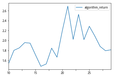
df6.index = df6['para1'].values
df6[['para1','algorithm_return']].plot()
<matplotlib.axes._subplots.AxesSubplot at 0x7f4fddf55a50>

#设定回测策略 id
# 注意!注意!注意!这里的id是在 我的策略里面的编译运行的algorithmId,在浏览器地址里面复制一下
pa = parameter_analysis('f50a271853f177b4d3d30b14eff6c7fe')
#运行回测
pa.get_backtest_data(file_name = 'results5.pkl',
                          running_max = 10,
                          benchmark_id = None,
                          start_date = '2008-12-05',
                           end_date = '2018-12-05',
                          frequency = 'day',
                          initial_cash = '100000000',
                          param_names = ['para1','para2'],
                          param_values = [['10','11','12','13','14','15','16','17','18','19','20','21','22','23','24','25','26','27','28','30'],[3]]
                          )
【已完成|运行中|待运行】: [0|0|20]. [0|10|10]. [3|7|10]. [已用0.022时,尚余0.022时,请不要关闭浏览器]. [10|3|7]. [12|8|0]. [13|7|0].
【回测完成】总用时:214秒(即0.06小时)。
#数据读取
pa.read_backtest_data('results5.pkl')
#查看回测结果指标
df5 = pa.evaluations_df
df5
| para1 | para2 | __version | algorithm_return | algorithm_volatility | alpha | annual_algo_return | annual_bm_return | avg_position_days | avg_trade_return | ... | max_drawdown_period | max_leverage | period_label | profit_loss_ratio | sharpe | sortino | trading_days | treasury_return | win_count | win_ratio | |
|---|---|---|---|---|---|---|---|---|---|---|---|---|---|---|---|---|---|---|---|---|---|
| 0 | 10 | 3 | 101 | 1.53432 | 0.181471 | 0.0418539 | 0.100268 | 0.0848782 | NaN | NaN | ... | [2015-06-12, 2018-12-05] | 0 | 2018-12 | NaN | 0.332107 | 0.402474 | 2433 | 0.400219 | NaN | NaN |
| 1 | 11 | 3 | 101 | 1.80154 | 0.183105 | 0.0528804 | 0.111659 | 0.0848782 | 1361 | 0.00707919 | ... | [2015-06-12, 2018-12-05] | 0 | 2018-12 | 1.39735 | 0.391357 | 0.473785 | 2433 | 0.400219 | 66 | 0.338462 |
| 2 | 12 | 3 | 101 | 1.85139 | 0.181915 | 0.0550891 | 0.113676 | 0.0848782 | 1361 | 0.00750812 | ... | [2015-06-12, 2018-12-05] | 0 | 2018-12 | 1.43433 | 0.405001 | 0.488552 | 2433 | 0.400219 | 64 | 0.338624 |
| 3 | 13 | 3 | 101 | 1.95747 | 0.183435 | 0.0588877 | 0.117864 | 0.0848782 | 1366 | 0.00807861 | ... | [2015-06-12, 2018-12-05] | 0 | 2018-12 | 1.49935 | 0.424475 | 0.513215 | 2433 | 0.400219 | 58 | 0.324022 |
| 4 | 14 | 3 | 101 | 1.94683 | 0.183724 | 0.0584149 | 0.11745 | 0.0848782 | 1361 | 0.008254 | ... | [2015-11-25, 2018-11-30] | 0 | 2018-12 | 1.54831 | 0.421555 | 0.510287 | 2433 | 0.400219 | 54 | 0.313953 |
| 5 | 15 | 3 | 101 | 1.71114 | 0.183796 | 0.0488681 | 0.107919 | 0.0848782 | 1363 | 0.0079412 | ... | [2015-06-12, 2018-11-30] | 0 | 2018-12 | 1.50483 | 0.369534 | 0.44506 | 2433 | 0.400219 | 49 | 0.291667 |
| 6 | 16 | 3 | 101 | 1.47948 | 0.183381 | 0.0388361 | 0.0977972 | 0.0848782 | 1366 | 0.00781405 | ... | [2015-06-12, 2018-11-30] | 0 | 2018-12 | 1.44679 | 0.315175 | 0.377609 | 2433 | 0.400219 | 46 | 0.289308 |
| 7 | 17 | 3 | 101 | 1.52717 | 0.183432 | 0.0410611 | 0.099948 | 0.0848782 | 1368 | 0.00817243 | ... | [2015-06-12, 2018-11-30] | 0 | 2018-12 | 1.45932 | 0.326813 | 0.39168 | 2433 | 0.400219 | 45 | 0.292208 |
| 8 | 18 | 3 | 101 | 1.84575 | 0.180868 | 0.055009 | 0.113449 | 0.0848782 | 1364 | 0.00892756 | ... | [2015-11-25, 2018-11-30] | 0 | 2018-12 | 1.59759 | 0.406093 | 0.491404 | 2433 | 0.400219 | 46 | 0.298701 |
| 9 | 19 | 3 | 101 | 1.6635 | 0.180882 | 0.0474507 | 0.105903 | 0.0848782 | 1366 | 0.00846828 | ... | [2015-11-25, 2018-11-30] | 0 | 2018-12 | 1.5479 | 0.36434 | 0.440149 | 2433 | 0.400219 | 45 | 0.294118 |
| 10 | 20 | 3 | 101 | 2.20461 | 0.181194 | 0.0685876 | 0.12712 | 0.0848782 | 1367 | 0.0105176 | ... | [2015-11-25, 2018-11-30] | 0 | 2018-12 | 1.64558 | 0.480813 | 0.582654 | 2433 | 0.400219 | 39 | 0.272727 |
| 11 | 21 | 3 | 101 | 2.69223 | 0.183037 | 0.0847354 | 0.143645 | 0.0848782 | 1374 | 0.0121224 | ... | [2015-11-25, 2018-11-26] | 0 | 2018-12 | 1.70167 | 0.566249 | 0.688305 | 2433 | 0.400219 | 38 | 0.279412 |
| 12 | 22 | 3 | 101 | 2.02202 | 0.183182 | 0.0614396 | 0.120347 | 0.0848782 | 1373 | 0.0109319 | ... | [2015-06-12, 2018-11-26] | 0 | 2018-12 | 1.52003 | 0.438617 | 0.531152 | 2433 | 0.400219 | 36 | 0.270677 |
| 13 | 23 | 3 | 101 | 2.52702 | 0.183497 | 0.0793642 | 0.138278 | 0.0848782 | 1370 | 0.013731 | ... | [2015-11-25, 2018-12-05] | 0 | 2018-12 | 1.66611 | 0.535581 | 0.651291 | 2433 | 0.400219 | 34 | 0.267717 |
| 14 | 24 | 3 | 101 | 2.0179 | 0.186289 | 0.060799 | 0.120189 | 0.0848782 | 1370 | 0.0126466 | ... | [2015-11-25, 2018-12-05] | 0 | 2018-12 | 1.50178 | 0.430458 | 0.517689 | 2433 | 0.400219 | 34 | 0.269841 |
| 15 | 25 | 3 | 101 | 2.28683 | 0.187264 | 0.070472 | 0.130058 | 0.0848782 | 1368 | 0.0139336 | ... | [2015-06-12, 2018-12-05] | 0 | 2018-12 | 1.58324 | 0.480917 | 0.57636 | 2433 | 0.400219 | 34 | 0.290598 |
| 16 | 26 | 3 | 101 | 2.09463 | 0.187018 | 0.0635644 | 0.123083 | 0.0848782 | 1364 | 0.0131264 | ... | [2015-06-12, 2018-12-05] | 0 | 2018-12 | 1.52505 | 0.444252 | 0.532583 | 2433 | 0.400219 | 33 | 0.275 |
| 17 | 27 | 3 | 101 | 1.88055 | 0.186435 | 0.0554284 | 0.114841 | 0.0848782 | 1365 | 0.013034 | ... | [2015-06-12, 2018-12-05] | 0 | 2018-12 | 1.53161 | 0.40143 | 0.4784 | 2433 | 0.400219 | 33 | 0.289474 |
| 18 | 28 | 3 | 101 | 1.79408 | 0.188034 | 0.0515226 | 0.111355 | 0.0848782 | 1371 | 0.0129666 | ... | [2015-06-12, 2018-12-05] | 0 | 2018-12 | 1.47497 | 0.379479 | 0.452258 | 2433 | 0.400219 | 31 | 0.27193 |
| 19 | 30 | 3 | 101 | 1.81217 | 0.186937 | 0.0525923 | 0.112092 | 0.0848782 | 1370 | 0.0134375 | ... | [2015-06-12, 2018-12-05] | 0 | 2018-12 | 1.55633 | 0.38565 | 0.459733 | 2433 | 0.400219 | 32 | 0.293578 |
20 rows × 28 columns
#7 回报率折线图
pa.plot_returns()

#指标回测收益列表
df5 = df5[['para1','para2','algorithm_return','alpha','sharpe','win_ratio','max_drawdown_period']]
df5.sort_values('algorithm_return',ascending=0)
| para1 | para2 | algorithm_return | alpha | sharpe | win_ratio | max_drawdown_period | |
|---|---|---|---|---|---|---|---|
| 4 | 21 | 3 | 2.69223 | 0.0847354 | 0.566249 | 0.279412 | [2015-11-25, 2018-11-26] |
| 5 | 23 | 3 | 2.52702 | 0.0793642 | 0.535581 | 0.267717 | [2015-11-25, 2018-12-05] |
| 6 | 25 | 3 | 2.28683 | 0.070472 | 0.480917 | 0.290598 | [2015-06-12, 2018-12-05] |
| 7 | 27 | 3 | 1.88055 | 0.0554284 | 0.40143 | 0.289474 | [2015-06-12, 2018-12-05] |
| 8 | 30 | 3 | 1.81217 | 0.0525923 | 0.38565 | 0.293578 | [2015-06-12, 2018-12-05] |
| 0 | 11 | 3 | 1.80154 | 0.0528804 | 0.391357 | 0.338462 | [2015-06-12, 2018-12-05] |
| 1 | 15 | 3 | 1.71114 | 0.0488681 | 0.369534 | 0.291667 | [2015-06-12, 2018-11-30] |
| 3 | 19 | 3 | 1.6635 | 0.0474507 | 0.36434 | 0.294118 | [2015-11-25, 2018-11-30] |
| 2 | 17 | 3 | 1.52717 | 0.0410611 | 0.326813 | 0.292208 | [2015-06-12, 2018-11-30] |
df5.index = df5['para1'].values
df5[['para1','algorithm_return']].plot()
<matplotlib.axes._subplots.AxesSubplot at 0x7f234ff7f490>


本社区仅针对特定人员开放
查看需注册登录并通过风险意识测评
5秒后跳转登录页面...
移动端课程